https://albertoarena.it/images/posts/php-is-not-dead-here-is-what-people-shipped/cover.jpg
Please wait while your request is being verified…
Laravel News Links
Just another WordPress site
https://albertoarena.it/images/posts/php-is-not-dead-here-is-what-people-shipped/cover.jpg
Please wait while your request is being verified…
Laravel News Links
https://gizmodo.com/app/uploads/2025/12/plex-1280×852.jpg
Plex shipped a security update in August that closed a chain of bugs letting anyone who can reach an exposed Plex Media Server run code on it. In one detailed public account, a hobbyist who later stood up a vulnerable server as a honeypot says attackers used that same chain on Saturday to drop a crypto miner and residential proxy software that lets other people route their traffic through a victim’s home internet connection, essentially using it as a VPN without the victim’s knowledge.
The bugs were originally found by a security researcher who goes by ZM online. In a technical write-up published Thursday, ZM described an unauthenticated remote code execution chain he calls Plex2Shell. In short, an attacker with no real login can trick a server into handing over its owner’s admin token, then plant a malicious file that runs the next time Plex transcodes a video. The chain strings together four vulnerabilities tracked as CVE-2026-96652, CVE-2026-96654, CVE-2026-96655, and CVE-2026-96656. Affected servers are those running versions before 1.43.3.10861.
ZM reported the issue to Plex on July 27th. Plex acknowledged it and paid a $500 bug bounty on August 4th, the same day the fixed build became publicly available to download. On September 1st, Plex posted a public advisory and, according to BleepingComputer, emailed users still on older versions. “We recommend all server owners and Desktop users update to the latest version as soon as possible,” Plex wrote. The company also said it had requested CVEs, which were assigned on September 23.
“Unauthenticated RCE chain in Plex,” ZM posted alongside the writeup and proof-of-concept code. “Patch your servers!” The $500 payout for such a critical exploit was immediately criticized, with multiple X users asking whether ZM had forgotten some zeros on the payout amount.
At the same time, an anonymous blogger who runs boredhackerblog had been waiting for those details to be revealed. “As an infosec person and a Plex user, I was really curious about what this vuln was and if I could see in-the-wild exploitation,” he wrote. He spun up a honeypot on an old Plex build. “As of this morning (Oct 17th), I finally saw in the wild exploitation using exploit code from the authors github,” they reported Saturday. The first payload was a crypto miner. Later the same day, they also saw a tool called myawesomeproxy, which prints a notice that running it means agreeing to “the potential external use of your internet traffic.” In other words, the attackers were turning the box into a residential proxy, the kind that other hackers rent to look like ordinary traffic while also masking their own IP addresses.
Kraken Chief Security Officer Nick Percoco cited the honeypot attack in an X post on Sunday. “If you run Plex at home, update it today,” he wrote, adding, “The payload sits in Plex’s Codecs folder and runs again every time something transcodes, so killing the miner doesn’t fix it.”
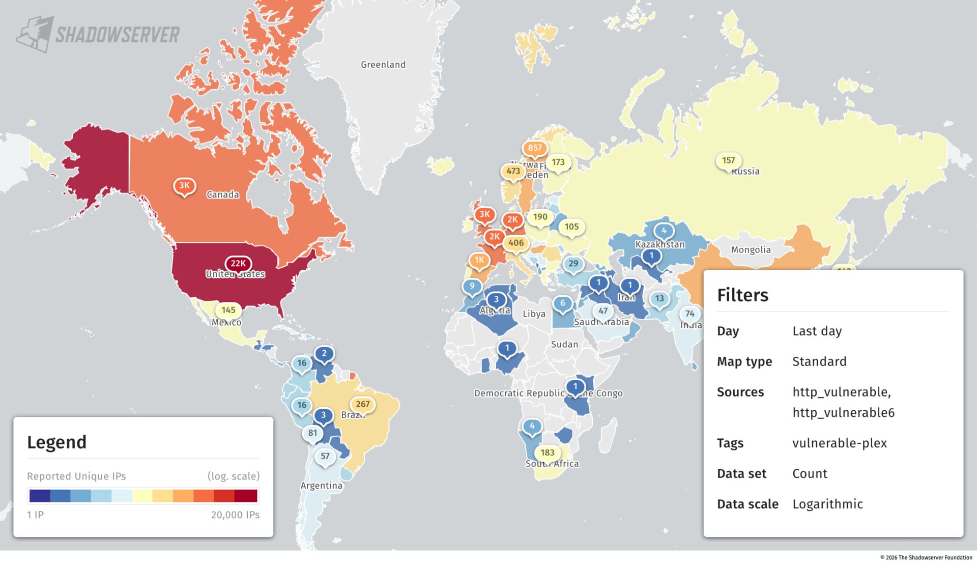
Plenty of people still have not patched their Plex servers. Shadowserver data on hosts tagged vulnerable-plex shows nearly 49,000 still exposed as of Saturday, including about 25,100 in North America and about 17,600 in Europe.
Plex has had its fair share of security incidents over the years. In September 2025, Plex told users to reset their passwords after an unauthorized party accessed emails, usernames, and hashed passwords. A month earlier, after a separate bug bounty report, Plex emailed users and told them to update to version 1.42.1. Weeks later, with many servers still vulnerable, it went further. “As a follow-up to the original report and in an abundance of caution due to a population of servers still on an affected Plex Media Server version (versions 1.41.7.x to 1.42.0.x), we have made adjustments for access to affected servers,” Plex wrote. “Specifically, other users to which the server owner has granted access to the server will not be able to connect to it while the server is running an affected version.” That flaw is now tracked as CVE-2025-34158.
Plex did not apply a similar access restriction, or otherwise require the update, after Plex2Shell became public. Its September 1st notice recommended an update and pointed Windows and Mac users at an optional automatic-update setting. That setting defaults to “Ask me,” not to auto-install, and Plex’s own support docs say it only applies to Windows and macOS. Linux, Docker, and NAS installs depend on package managers, container restarts, or manual downloads. Plex’s terms of service say the company can require an update “as a means to protect the Plex Solution from unauthorized use, content, or data,” and that declining one may cut off access. As of Sunday afternoon Eastern time, Plex had also not issued any new public statement about the exploit or the attacks that followed it.
A previous LastPass hack also shows that the stakes involved with this kind of vulnerability in Plex server software can be quite high. In 2023, LastPass said attackers got into a senior DevOps engineer’s home computer “by targeting the DevOps engineer’s home computer and exploiting a vulnerable third-party media software package, which enabled remote code execution capability and allowed the threat actor to implant keylogger malware,” according to Ars Technica. Ars reported that a person briefed on a private LastPass report identified the package as Plex; however, LastPass and Plex have not publicly confirmed that link in matching detail. Either way, it is the nightmare version of what a vulnerable residential Plex server can become when a remote code execution exploit is discovered.
Gizmodo
https://percona.community/blog/2026/10/pgsm-2-4-0-cover_hu_17d1ca2b2c9b78d0.jpg
pg_stat_monitor started as a fork of pg_stat_statements, built to be a more advanced replacement for it. It provides more detailed information about query execution and groups it in configurable time buckets, so you can look at what happened in a particular time window. It also powers the Query Analytics feature in Percona Monitoring and Management (PMM). However, over time other work took priority at Percona, and the extension stopped getting the attention it needed. The original developers moved on to other things, and the reasoning behind several design decisions went with them. For a couple of years it stayed in maintenance mode, we were fixing reported bugs, and never stepped back to look at deep architectural issues. All that led to a degraded user experience and stability issues.
2.4.0 is our attempt to turn that around. It is the biggest release in years: about 250 commits since 2.3.2. We restructured the code and fixed bugs across the whole extension, and the C code got about 20% smaller. Among the fixes are several buffer overflows, a use-after-free, a lock ordering problem and a few statistics that were simply wrong. We also backported the pg_stat_statements regression tests. The most important fixes, though, are about memory management, and that is what this post is about. For everything else, see the release notes.
Well, memory leaked under certain workloads. The end was always the same: the process eventually got killed by the OOM killer.
Not every workload was affected, it depended on how it was run. Queries sent over the simple protocol were fine. Named prepared statements leaked memory on every execution. Statements running through SPI inside a background worker leaked the same way. In both cases nothing reclaimed the memory, so growth stopped only when the session or the worker did.
Another problematic case is when statements produce warnings. On PostgreSQL 18 and earlier, each warning caused a small memory leak, which could accumulate over time if many warnings were generated.
Server code does not call malloc() and free() directly. Instead it uses memory contexts, also known as memory arenas outside PostgreSQL. Every allocation happens within a context, and freeing the context releases all allocated memory at once. Contexts form a tree structure, so freeing a parent context frees every child context as well. This is what lets PostgreSQL manage memory efficiently and survive an error thrown in the middle of a query.
So when you write an extension, you should keep in mind which context your allocations belong to and when that context will be freed.
Four contexts matter for our topic:
TopMemoryContext is the root context for the backend. It lives as long as the backend does and is only destroyed when the backend exits.TopTransactionContext is reset at every commit and every abort, which deletes all of its child contexts.MessageContext is reset after each client protocol message.ErrorContext is reserved for error reporting. On PostgreSQL 18 and earlier, it is only reset during error recovery.An extension can create its own context or use one of the existing ones. Choosing a context with the wrong lifetime causes problems: your data either vanishes too early or stays around longer than needed. The latter looks exactly like a leak, even though every byte is still accounted for.
pg_stat_monitor collects per-statement statistics in backend-local memory first, and dumps them into the shared time buckets when the statement finishes and we have the full set of data. That local memory lived in a context called PgsmMemoryContext, and it was created as a child of TopMemoryContext. TopMemoryContext lives as long as the backend does. So instead of relying on context lifetime, pg_stat_monitor used a persistent context, and for cleanup it used a reset callback assigned to another context: MessageContext. MessageContext is reset after every client protocol message, and a reset invokes the callback, which cleaned out PgsmMemoryContext without destroying it.
One detail matters for everything below. A reset callback in PostgreSQL is one-shot: it is popped off the context’s callback list before it is called, so it fires once and is gone. To keep the cleanup working, pg_stat_monitor had to register a fresh callback for every message. It did this from the post parse analyze hook, one of the first steps in the statement lifecycle. So callback setup depends not on the statement finishing, but on the next message going through parse analysis. This design has two weak points, and we hit both of them.
Background workers have no MessageContext. So a statement running through SPI inside a background worker never arms the reset callback at all. Nothing resets PgsmMemoryContext, and because its parent is TopMemoryContext, nothing else is going to. It keeps growing for the life of the worker.
In the extended query protocol, the client sends a named prepared statement as separate messages: Parse once, then Bind and Execute for every run. Parse analysis happens only during Parse, so that is the only message that arms the callback. When MessageContext is reset after Parse, the callback fires and nothing re-arms it. MessageContext is still reset after every Bind and Execute, but no callback is attached to it anymore, so PgsmMemoryContext keeps growing for the life of the session. This is the pattern database drivers use for prepared statements. Note that the SQL-level PREPARE and EXECUTE commands are not affected, because each EXECUTE statement goes through parse analysis itself and re-arms the callback.
pg_stat_monitor records the warnings and errors a statement produces, so it hooks into the code PostgreSQL uses to emit log messages. That hook runs in the middle of error reporting, and error reporting has a memory context of its own, ErrorContext. PostgreSQL keeps that one reserved so it always has somewhere to build a message, even when the backend is short on memory. It is cleaned out when the server unwinds from an error. A WARNING does not unwind anything: the statement simply carries on. PostgreSQL 19 added ErrorContext resets after reporting a warning, so this leak only affects PostgreSQL 18 and earlier.
Our hook copied the query text wherever it happened to be running, so that copy landed in ErrorContext instead of in pg_stat_monitor’s own context. Nothing was ever going to reclaim it. The entry for the statement itself went to PgsmMemoryContext, so it stayed there until the next MessageContext reset cleaned it up, if that ever happened.
Both problems come from the same place. We inherited the design from pg_stat_statements, which we forked years ago, and we never revisited it as pg_stat_monitor grew code paths that upstream does not have. The test suite did not help either. We had nothing that ran a background worker in a loop, nothing that held a session open across thousands of Bind and Execute cycles, and nothing that measured backend memory at all. None of this is exotic.
Both problems have the same shape. The memory sat in a context that never dies, and the cleanup depended on an event that does not always happen. Rather than trying to make the cleanup callback fire on every path, we changed where the memory lives.
Every path that can execute a statement runs inside a transaction. Background worker SPI, named prepared statements, ordinary queries. A background worker may not have a MessageContext, but it always has a transaction.
The change is:
PgsmMemoryContext is no longer a child of TopMemoryContext. It is created as a child of TopTransactionContext, so it is automatically deleted at every commit and every abort. There is no callback to register and nothing to re-arm, so there is no execution path left that can skip the cleanup.ErrorContext allocations completely.This covers all three cases from the beginning of the post. A background worker always runs its statements inside a transaction, so its memory is now freed when that transaction ends, the same as in a regular backend. Named prepared statements no longer depend on parse analysis to clean up after them, every Execute is followed by a commit that frees the memory. Warnings no longer allocate anything that outlives the hook.
2.4.0 was about stabilizing the code base we already have. We reworked memory management, removed code we no longer need, and built the test coverage that should have been there from the start. We did not change how the extension is structured. That is the plan for the next major release: we want to revisit the architecture of pg_stat_monitor, starting with how it uses shared memory and how it behaves when that memory fills up. ∎
Planet for the MySQL Community
It already has a port just on just about every hardware platform released in the last decade, and now there’s finally an unofficial one for Mac. The new vibecoded SkyrimMT project is a one-click installer to get and install everything you need to play the title, with mods, on your Apple Silicon Mac. I’ve only tested it for a few minutes this morning, but it runs great on a M1 MacBook Air.
Continue Reading on AppleInsider | Discuss on our ForumsAppleInsider News
https://media.babylonbee.com/articles/6ace7c41bad0f6ace7c41bad10.jpg
HARAN — Following a night of wine and music, Jacob reportedly began to assure his new bride Rachel that he hadn’t gotten that drunk at the wedding last night, only to discover he had, in fact, gotten that drunk.
According to new information, Jacob had not married Rachel the night before as previously intended, but he had instead gotten totally smashed and then married her sister Leah.
Leah, who had not overindulged the night before, was reportedly offended when her new husband kept saying, "Oh no, oh no, oh no! This can’t be happening! Where’s Rachel? WHERE’S RACHEL?"
Laban, the father of Leah and Rachel, was suspected of intentionally bullying Jacob into taking shots of tequila as part of a scheme to marry off his eldest daughter first.
"Yeah, he worked seven years for Rachel, but have you seen Leah?" Laban said by way of defense. "I had to get her a husband somehow."
Rachel later said of the matter, "It’s fine."
At publishing time, Jacob agreed to work seven more years for Rachel if Laban would promise not to get him drunk and marry him to one of his camels.
Noah’s Ark has definitely been found and we highlight 9 incredible artifacts that prove it.
Babylon Bee
https://percona.community/blog/2026/10/dba_docker_lab_hu_d6c3281482a4c3e5.jpg
How I built a local database playground, learned a few lessons the hard way, and created a practical command reference along the way.
One of the best ways to learn database administration is to get your hands dirty.
Documentation is important, but there’s something different about building your own environment, breaking it, troubleshooting it, and eventually understanding why everything works.
Recently, I decided to create a local database lab using Docker Desktop on my Mac. My goal was straightforward: build an environment where I could experiment with MySQL, PostgreSQL, Percona XtraDB Cluster (PXC), and Percona Monitoring and Management (PMM), without worrying about disrupting a production environment.
What started as a few containers quickly became a much more interesting learning experience.
Along the way, I ran into Docker networking problems, container persistence challenges, cluster bootstrap issues, and PostgreSQL monitoring configuration. This article shows the setup I recommend after working through those problems, so you can start with the right foundation instead of discovering it at the end.
The foundation of my environment is Docker Desktop.
The lab includes:
The architecture looks like this:
text
Docker Desktop
│
├── pmm-network
│ ├── pmm-server
│ ├── pmm-client
│ ├── percona-server
│ ├── postgres-server
│ ├── pxc1
│ ├── pxc2
│ └── pxc3
│
└── Persistent Docker Volumes
 ├── pmm-data
 ├── pmm-client-data
 ├── mysql-data
 ├── postgres-data
 ├── pxc1_data
 ├── pxc2_data
 └── pxc3_data
There are two ways to build this.
Docker Compose lets you define every container, volume, and network attachment in one file. The whole lab becomes reproducible: one command brings it up, one command shuts it down, and nothing depends on remembering which docker run flags you used weeks ago.
I started out with individual docker run commands and later moved everything to Compose. If I were starting again, I would begin here.
First, keep passwords out of the Compose file by putting them in a .env file next to it (and out of version control):
bash
# .env
MYSQL_ROOT_PASSWORD=change-me
PXC_ROOT_PASSWORD=change-me
POSTGRES_PASSWORD=change-me
PMM_ADMIN_PASSWORD=change-me
PG_MONITOR_PASSWORD=change-me
MYSQL_MONITOR_PASSWORD=change-me
Then define the lab in docker-compose.yml:
yaml
services:
 pmm-server:
 image: percona/pmm-server:3.9.1
 platform: linux/amd64
 container_name: pmm-server
 ports:
 - "443:8443"
 volumes:
 - pmm-data:/srv
 networks: [pmm-network]

 pmm-client:
 image: percona/pmm-client:3.9.1
 container_name: pmm-client
 depends_on: [pmm-server]
 environment:
 PMM_AGENT_SERVER_ADDRESS: pmm-server:8443
 PMM_AGENT_SERVER_USERNAME: admin
 PMM_AGENT_SERVER_PASSWORD: ${PMM_ADMIN_PASSWORD}
 PMM_AGENT_SERVER_INSECURE_TLS: 1
 PMM_AGENT_SETUP: 1
 PMM_AGENT_CONFIG_FILE: config/pmm-agent.yaml
 volumes:
 - pmm-client-data:/usr/local/percona/pmm/config
 networks: [pmm-network]

 percona-server:
 image: percona/percona-server:8.4.11
 container_name: percona-server
 environment:
 MYSQL_ROOT_PASSWORD: ${MYSQL_ROOT_PASSWORD}
 ports:
 - "3306:3306"
 volumes:
 - mysql-data:/var/lib/mysql
 networks: [pmm-network]

 postgres-server:
 image: postgres:17
 container_name: postgres-server
 environment:
 POSTGRES_PASSWORD: ${POSTGRES_PASSWORD}
 command: >
 postgres
 -c shared_preload_libraries=pg_stat_statements
 -c track_io_timing=on
 ports:
 - "5432:5432"
 volumes:
 - postgres-data:/var/lib/postgresql/data
 networks: [pmm-network]

 pxc1:
 image: percona/percona-xtradb-cluster:8.4.11
 container_name: pxc1
 environment:
 CLUSTER_NAME: pxc-lab
 MYSQL_ROOT_PASSWORD: ${PXC_ROOT_PASSWORD}
 volumes:
 - pxc1_data:/var/lib/mysql
 - ./certs:/etc/mysql/certs:ro
 - ./conf.d:/etc/percona-xtradb-cluster.conf.d:ro
 stop_grace_period: 120s
 healthcheck:
 test: ["CMD", "mysqladmin", "ping", "-uroot", "-p${PXC_ROOT_PASSWORD}"]
 interval: 10s
 retries: 30
 networks: [pmm-network]
 ports:
 - "3307:3306"

 pxc2:
 image: percona/percona-xtradb-cluster:8.4.11
 container_name: pxc2
 environment:
 CLUSTER_NAME: pxc-lab
 CLUSTER_JOIN: pxc1
 MYSQL_ROOT_PASSWORD: ${PXC_ROOT_PASSWORD}
 volumes:
 - pxc2_data:/var/lib/mysql
 - ./certs:/etc/mysql/certs:ro
 - ./conf.d:/etc/percona-xtradb-cluster.conf.d:ro
 stop_grace_period: 120s
 depends_on:
 pxc1:
 condition: service_healthy
 networks: [pmm-network]
 ports:
 - "3308:3306"

 pxc3:
 image: percona/percona-xtradb-cluster:8.4.11
 container_name: pxc3
 environment:
 CLUSTER_NAME: pxc-lab
 CLUSTER_JOIN: pxc1
 MYSQL_ROOT_PASSWORD: ${PXC_ROOT_PASSWORD}
 volumes:
 - pxc3_data:/var/lib/mysql
 - ./certs:/etc/mysql/certs:ro
 - ./conf.d:/etc/percona-xtradb-cluster.conf.d:ro
 stop_grace_period: 120s
 depends_on:
 - pxc2
 networks: [pmm-network]
 ports:
 - "3309:3306"

networks:
 pmm-network:
 name: pmm-network

volumes:
 pmm-data:
 pmm-client-data:
 mysql-data:
 postgres-data:
 pxc1_data:
 pxc2_data:
 pxc3_data:
A few design choices are worth calling out, because each one comes from a problem I hit:
pmm-network from the moment it is created, so there is nothing to wire up afterward.stop_grace_period: 120s gives each PXC node time to shut down cleanly instead of being killed (exit code 137).depends_on defines the PXC order. Compose starts pxc1 first and waits for it to be healthy before the others join. On shutdown, Compose stops dependents first, so the nodes leave in the order pxc3, pxc2, pxc1.Bring the lab up and down with:
bash
docker compose up -d
docker compose stop # stops containers, keeps everything
docker compose down # removes containers, keeps named volumesdocker run commandsIf you prefer to build containers one at a time, or want to understand what Compose is doing for you, you can create the network yourself and attach containers to it:
bash
docker network create pmm-network

docker run -d --name postgres-server \
 --network pmm-network \
 -e POSTGRES_PASSWORD="$POSTGRES_PASSWORD" \
 -v postgres-data:/var/lib/postgresql/data \
 -p 5432:5432 \
 postgres:17
An existing container can be attached later:
bash
docker network connect pmm-network postgres-serverThis works, but you are responsible for recreating each container with exactly the same flags, volumes, and network settings every time. That is the main reason I recommend Option A. Whichever option you choose, avoid mixing the two for the same lab, because it becomes hard to tell which containers are managed by Compose and which are not.
At one point, PMM couldn’t resolve my PostgreSQL container:
text
lookup postgres-server on 127.0.0.11:53: no such hostThe problem wasn’t PostgreSQL or PMM. The PostgreSQL container was stopped, so it had no active network endpoint, and Docker’s internal DNS had nothing to return.
That was an important reminder: always verify the container and network state before troubleshooting the application.
Once the databases were running, I wanted visibility into their performance.
PMM provides dashboards and metrics for MySQL, PXC, and PostgreSQL. It consists of a server that stores and visualizes monitoring data and a client agent that collects database metrics.
The key thing to understand is that persistent storage and service registration are related, but they are not the same thing.
PMM Server maintains the monitoring inventory, while PMM Client has its own configuration and agent identity. If the client is recreated with a new identity, the association between the client and its registered services is lost. In my early setup, after recreating containers, the client listing showed only the basic agents:
text
pmm_agent Connected
node_exporter Running
vmagent Running
Two things prevent this, and both should be in place from the start:
pmm-client-data keeps the agent identity across restarts and recreations.docker compose up.Before registering, create a monitoring user in each database. For PostgreSQL, for example:
sql
CREATE USER pmm WITH PASSWORD 'change-me';
GRANT pg_monitor TO pmm;
CREATE EXTENSION IF NOT EXISTS pg_stat_statements;
Then the registration script, which reads credentials from the .env file rather than hardcoding them:
bash
#!/usr/bin/env bash
# register-pmm.sh
set -euo pipefail
source .env

registered() {
 docker exec pmm-client pmm-admin list | grep -qw "$1"
}

if ! registered postgres-server; then
 docker exec pmm-client pmm-admin add postgresql \
 --username=pmm \
 --password="$PG_MONITOR_PASSWORD" \
 --host=postgres-server \
 --port=5432 \
 postgres-server
fi

for node in percona-server pxc1 pxc2 pxc3; do
 if ! registered "$node"; then
 docker exec pmm-client pmm-admin add mysql \
 --username=pmm \
 --password="$MYSQL_MONITOR_PASSWORD" \
 --host="$node" \
 --port=3306 \
 --query-source=perfschema \
 "$node"
 fi
done

docker exec pmm-client pmm-admin list
The takeaway: a monitoring system should be designed to survive a restart, not just work immediately after installation.
With PostgreSQL running and connected to PMM, I wanted to do more than look at an idle dashboard.
I used sysbench to generate a workload against PostgreSQL 17.
My test environment included ten tables with approximately 750,000 rows each, giving me about 7.5 million rows to experiment with.
A sample workload command looked like this:
bash
sysbench \
 --db-driver=pgsql \
 --pgsql-host=127.0.0.1 \
 --pgsql-port=5432 \
 --pgsql-user=postgres \
 --pgsql-db=sbtest \
 --tables=10 \
 --table-size=750000 \
 --threads=16 \
 --time=300 \
 --report-interval=5 \
 oltp_read_write run
With the workload running, PMM became much more interesting.
I could observe database activity, disk latency, query execution statistics, and changes in resource utilization.
This also helped me understand an important distinction: PostgreSQL tuple activity is not the same thing as SQL queries per second.
One query can read or return many tuples. Looking only at tuple counts without understanding the underlying queries can lead to incorrect conclusions about workload intensity.
One of the most useful PostgreSQL features for troubleshooting is EXPLAIN.
For example:
sql
EXPLAIN (ANALYZE, BUFFERS)
SELECT *
FROM sbtest1
WHERE id BETWEEN 100 AND 200;
This shows the execution plan, actual execution measurements, and buffer activity.
I started paying attention to several key pieces of information:
Because the Compose file loads pg_stat_statements at startup, query statistics are aggregated from the beginning.
A useful query is:
sql
SELECT
 calls,
 total_exec_time,
 mean_exec_time,
 rows,
 LEFT(query, 100) AS query
FROM pg_stat_statements
ORDER BY total_exec_time DESC
LIMIT 10;
This provides a different perspective from looking at individual slow queries.
A query that takes only a fraction of a millisecond might still consume substantial cumulative execution time if it runs hundreds of thousands of times.
For a DBA, both individual latency and aggregate workload matter.
My next learning objective was understanding PostgreSQL’s Multi-Version Concurrency Control (MVCC).
Unlike an in-place overwrite model, PostgreSQL commonly creates a new row version when a row is updated.
Older versions may remain until PostgreSQL determines they are no longer needed.
That leads directly to one of PostgreSQL’s most important maintenance mechanisms: VACUUM.
I experimented with updating large numbers of rows:
sql
UPDATE sbtest1
SET k = k + 1
WHERE id <= 300000;
Then checked the table statistics:
sql
SELECT
 relname,
 n_live_tup,
 n_dead_tup,
 last_autovacuum,
 autovacuum_count
FROM pg_stat_user_tables
WHERE relname = 'sbtest1';
This gave me a practical way to observe dead tuple estimates and autovacuum activity.
I also explored what happens when a long-running transaction holds an old snapshot.
By starting a REPEATABLE READ transaction and leaving it open while another session updated rows, I could demonstrate how PostgreSQL may need to retain older row versions.
That helped connect several important DBA concepts:
Long-running transactions → old snapshots → delayed tuple cleanup → potential table bloat.
I also learned that normal VACUUM generally makes space reusable within PostgreSQL rather than immediately shrinking the table file.
VACUUM FULL can reclaim disk space by rewriting a table, but it requires an exclusive lock and is not something to run casually in production.
My three-node Percona XtraDB Cluster taught me that database containers need database-aware operational procedures. That’s why startup and shutdown are built into the Compose file rather than left to chance.
Early on, I ran into certificate problems, donor timeouts, cluster membership issues, and shutdowns that ended with exit code 137 (the container being killed before MySQL finished). The shared certificate directory, the healthcheck on pxc1, and stop_grace_period address those directly.
The shutdown procedure is simply:
bash
docker compose stop pxc3 pxc2 pxc1If you use Option B, do the same thing explicitly, one node at a time, with a long timeout:
bash
docker stop -t 120 pxc3
docker stop -t 120 pxc2
docker stop -t 120 pxc1
To start the cluster again, check grastate.dat on each node and understand the meaning of safe_to_bootstrap:
bash
docker run --rm -v pxc1_data:/data alpine cat /data/grastate.datAfter a clean shutdown, the last node to leave the cluster (here, pxc1) will have safe_to_bootstrap: 1 and is the right node to start first.
After an unclean shutdown, selecting the correct bootstrap node requires recovery checks. Compare the recovered sequence numbers across nodes and bootstrap from the most advanced one. Simply changing safe_to_bootstrap to 1 without verifying that can lose data.
I kept a command cheat sheet from the start of the project, and it has become one of the most useful outcomes. It captures the commands I actually needed while learning and troubleshooting. I recommend starting one on day one.
For Docker:
bash
# Running containers
docker ps

# All containers
docker ps -a

# Status of the Compose-managed lab
docker compose ps

# Follow logs
docker logs -f postgres-server

# Inspect network configuration
docker inspect postgres-server \
 --format ''

# Resource usage
docker stats

# List Docker volumes
docker volume ls

# Check PMM services
docker exec pmm-client pmm-admin list
These commands are my first line of investigation whenever something isn’t behaving as expected.
For PostgreSQL, my daily reference includes:
sql
-- Current sessions
SELECT pid, usename, state, query
FROM pg_stat_activity;

-- Long-running transactions
SELECT
 pid,
 state,
 now() - xact_start AS transaction_age,
 query
FROM pg_stat_activity
WHERE xact_start IS NOT NULL;

-- Dead tuples
SELECT relname, n_live_tup, n_dead_tup
FROM pg_stat_user_tables
ORDER BY n_dead_tup DESC;

-- Blocking sessions
SELECT
 pid,
 pg_blocking_pids(pid) AS blocked_by
FROM pg_stat_activity
WHERE cardinality(pg_blocking_pids(pid)) > 0;
These are simple queries, but they form a useful starting point for troubleshooting.
To summarize, these are the principles the setup above is built on:
docker run commands with Compose-managed containers.What began as an effort to build a small local database environment turned into a practical DBA learning experience.
I now have a place to explore PostgreSQL performance, MVCC, autovacuum, MySQL replication concepts, PXC clustering, and database monitoring without risking a production system.
Perhaps the biggest lesson is that the most valuable learning moments often happen when something breaks.
A Docker DNS failure teaches networking. A missing PMM registration teaches persistence and identity. A PXC bootstrap problem teaches cluster recovery. A growing dead tuple count teaches PostgreSQL MVCC.
And once you understand why something broke, you’re much better prepared to troubleshoot it the next time.
My next goal is to continue expanding the lab with PostgreSQL replication, backup and recovery, and more deliberate performance troubleshooting exercises.
This article describes a local learning environment. The commands and configurations are intended for experimentation and should be reviewed and adapted before use in production. ∎
Planet for the MySQL Community
https://blogger.googleusercontent.com/img/b/R29vZ2xl/AVvXsEjNOm1nV5-sOyOlra6B3XU3XpTycZ2Wbcxw6SMB48x6pnDd212OTqXwBaNEGXel4tkZzHWZa5YA_zr76jDSxdkoXSOwmiJJmQNYnscfyP7aqjCBkAbjAfZ5wFIU63iXnxuHInOKCAqZ88R_XJqGwNzrLHd44LzMiBw_byEJSKhIaa8-8-i7bEzgQav1SQqF/w1200-h630-p-k-no-nu/Screenshot%20From%202026-10-08%2010-49-02.png
The old MySQL Workbench was ‘retired’ in January. The latest was recent released without a lot of fanfare. The new version is not an evolution of the old and, in some ways, is lacking features like relationship maps and reverse engineering capabilities. Now server versions 8.0 and earlier may work, but are not supported.
 |
| The opening screen of the newest MySQL Workbench |
New Look
The new version is built on the top of MySQL Shell. A lot of the features from that product are still around, but the look and feel will not feel familiar to the fans of the shell.
By The Way: The MySQL Shell for VS Code has also been discontinued.
Installation can be made from any of the usual ways from the usual sources. This is still the high quality package we have come to expect.
 |
| What you see when you are working with SQL |
Connections are made from the first page by clicking on the plus ‘+’ button and providing the connection details.
From there click on the box with your connection name.
Now you can write queries to your heart’s content. You will have to click on the blue ‘Run’ button to get the query to execute. Or, use the Run menu.
The GUI is minimalist, to put it nicely.
Under the Run menu, you can ‘run’ the query and use Explain, either text or visual. The visual explain was a highlight of the previous version.
The auto-completion is improved, but other products were much better earlier.
I wanted to show examples of the visual explain, but I only received ‘No database selected’ messages. Supposedly it supports the hypergraph optimizer and specialized HeatWave Query plans. But not on a local instance with a query that ran well with the non-visual explain options. Frustrating.
Notebooks bring the ability to use JavaScript, TypeScript, or SQL to execute code blocks. This was popular in the MySQL Shell.
I liked the Python capabilities of the previous edition.
 |
| Notebooks provide for JavaScript, TypeScript, and SQL scripting |
Having to hit the Run button or use the Run menu to execute queries gets old very quickly.
Again, minimalist, and very thin compared to the older version. In this age of observation of all things being key, this is disappointing.
 |
| Server Status |
Well, the older version had a lot of interesting and sometimes quirky information on system performance.
 |
| Some performance information is available |
Prepared to be nostalgic again as they are missing from this new version. This an no ERM maps remove capabilities where Workbench used to be top notch.
I have to inform you that I am an employee of DBeaver, which is a competing product. Just as skipping is a competitor to a race car at the Indy 500.
This version of MySQL Workbench is too stark and minimalist in design for me. It lacks too many features.
And it is MySQL 8.0 (maybe) or later only.
I do not know if Oracle/MySQL will add features in the future. This new project is open-source, but will it attract developers to help improve it? Go into ‘not holding my breath mode’ for both cases here.
I will check back when there is a new release, but MySQl Workbench 26.7 is not going into my tool box.
Planet for the MySQL Community
https://media.notthebee.com/articles/6ac6a74a89f6e6ac6a74a89f6f.jpg
I AM DECEASED.
Not the Bee
We recently wrote about RemoveMacAI, a tool to disable Apple Intelligence and delete the models, to help save about 13 gigabytes of storage space. While it was initially provided as Terminal commands, you can now download an app that gives you a friendly UI to use.
Be aware that it isn’t a notarized app, so you’ll have a few more hoops to jump through to run it.
Continue Reading on AppleInsider | Discuss on our ForumsAppleInsider News
https://media.appleinsider.com/gallery/69262-146090-4B6E3B65-E64C-4F50-B420-A37E3F4428C4-xl.jpgSonnet’s Echo SE I T5 gives Mac mini and MacBook Pro users a way to add the kind of PCIe hardware normally reserved for larger workstations without giving up the compact Mac they already have.
 Sonnet’s Echo SE I T5
The Thunderbolt 5 enclosure supports video capture cards, professional audio hardware, RAID controllers, and high-speed networking adapters. Sonnet says the system can deliver up to 6,800 MB/s of bidirectional PCIe bandwidth over Thunderbolt 5.
Thunderbolt 5 gives demanding PCI-E cards substantially more bandwidth than older Thunderbolt connections can provide.
The Echo SE I T5 gives compact Macs a practical path to PCIe expansion without making bandwidth the whole story. Because the Mac mini and MacBook Pro don’t have internal PCIe slots, adding specialized hardware usually means using an external enclosure or moving to a larger workstation.
Continue Reading on AppleInsider | Discuss on our ForumsAppleInsider News