https://media.townhall.com/townhall/reu/o/2018/238/93bb559c-1119-49a5-b73c-c0aafefe3063-1110×740.jpg
A Factory That Makes Rice Cookers from Stone
https://theawesomer.com/photos/2022/09/making_rice_cookers_from_stone_t.jpg

Modern rice cookers are made from metal and plastic, but traditional Korean rice cookers are made from stone. This fascinating video from Factory Monster takes us inside a company that creates the bowl-shaped cookers and their lids by cutting them from a 9-ton boulder. The English subtitles are quite entertaining.
The Awesomer
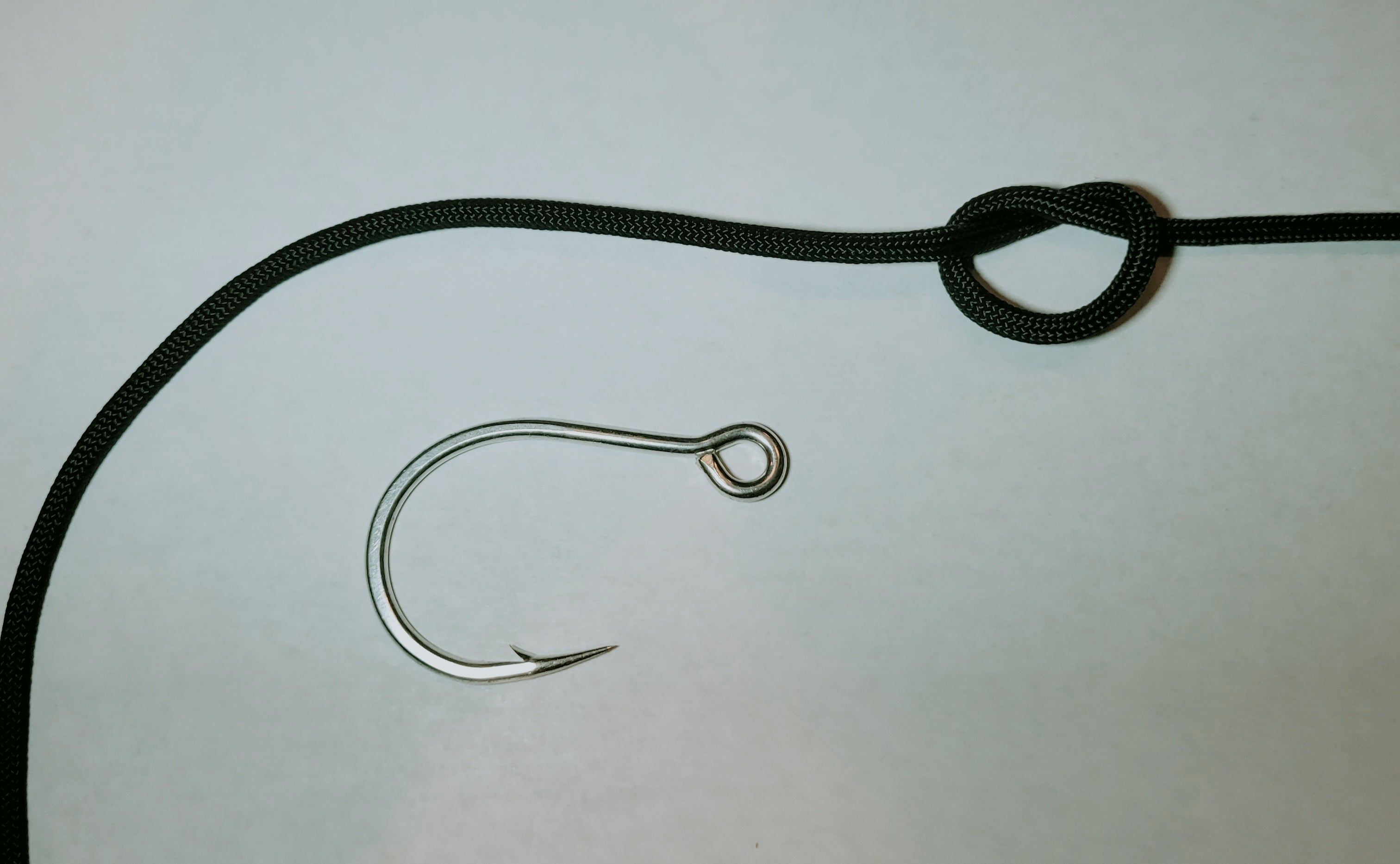
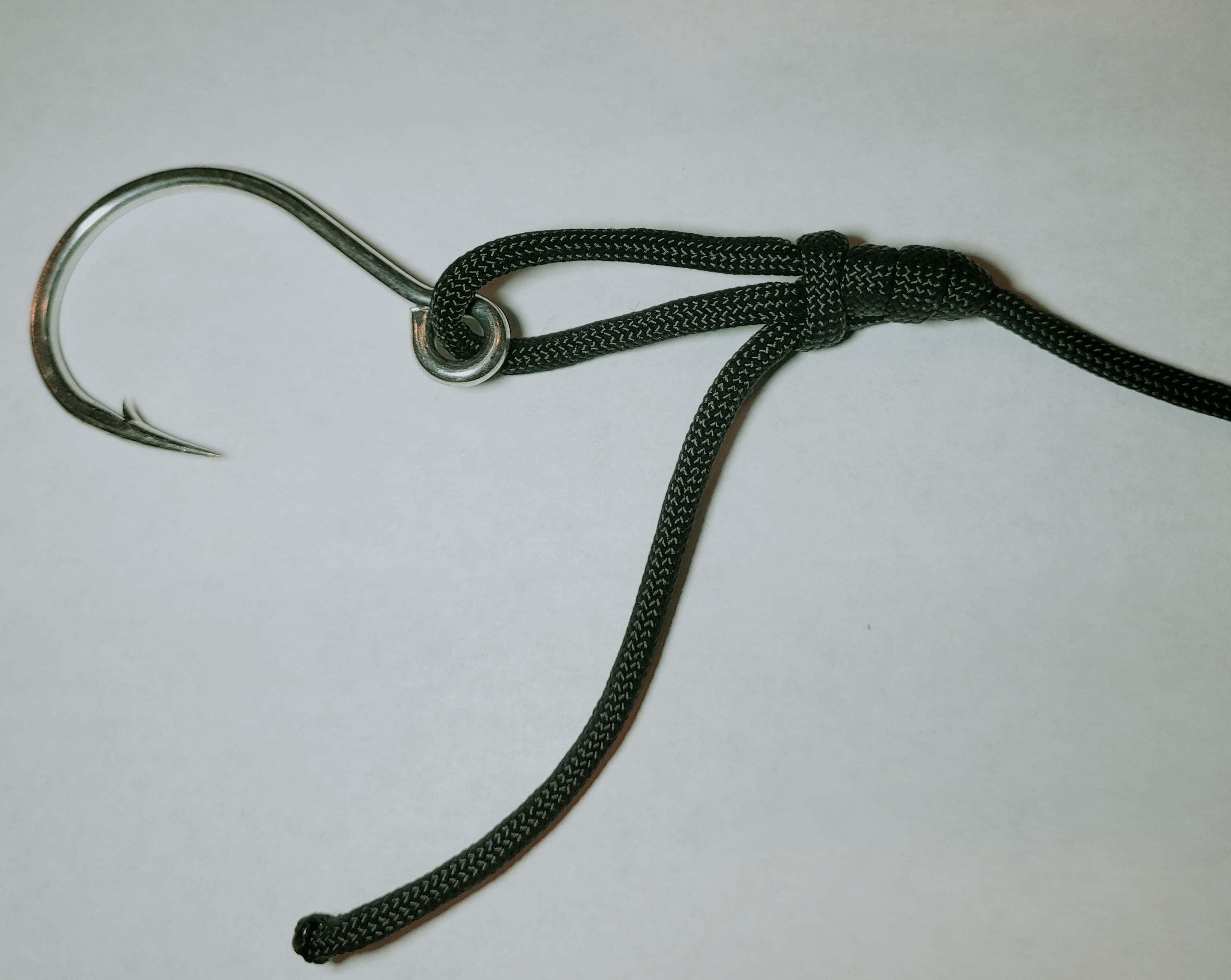
Are You Nuts? Know your Fishing Knots! – The Non-Slip Loop Knot
https://www.alloutdoor.com/wp-content/uploads/2022/09/20220920_171915.jpg
Last week we covered the Surgeon Knot, one of the quickest and easiest loop knots to tie. But there is a downside to that knot, it’s a bit bulky and especially in a more finesse presentation isn’t the best choice for anglers. This is especially true for fly anglers chasing after skittish trout. This is where the Non-Slip Loop Knot comes into the picture. This knot does take more effort to tie but will be a much neater knot once you’re finished with it. The Non-Slip Loop Knot has comparable strength to the Surgeon knot and works great for direct attachment to lures, jigs, and flies.
Step 1
Get your mainline and tie an overhand knot in it, making sure to have a decent length of tag end left for tying the rest of the knot.
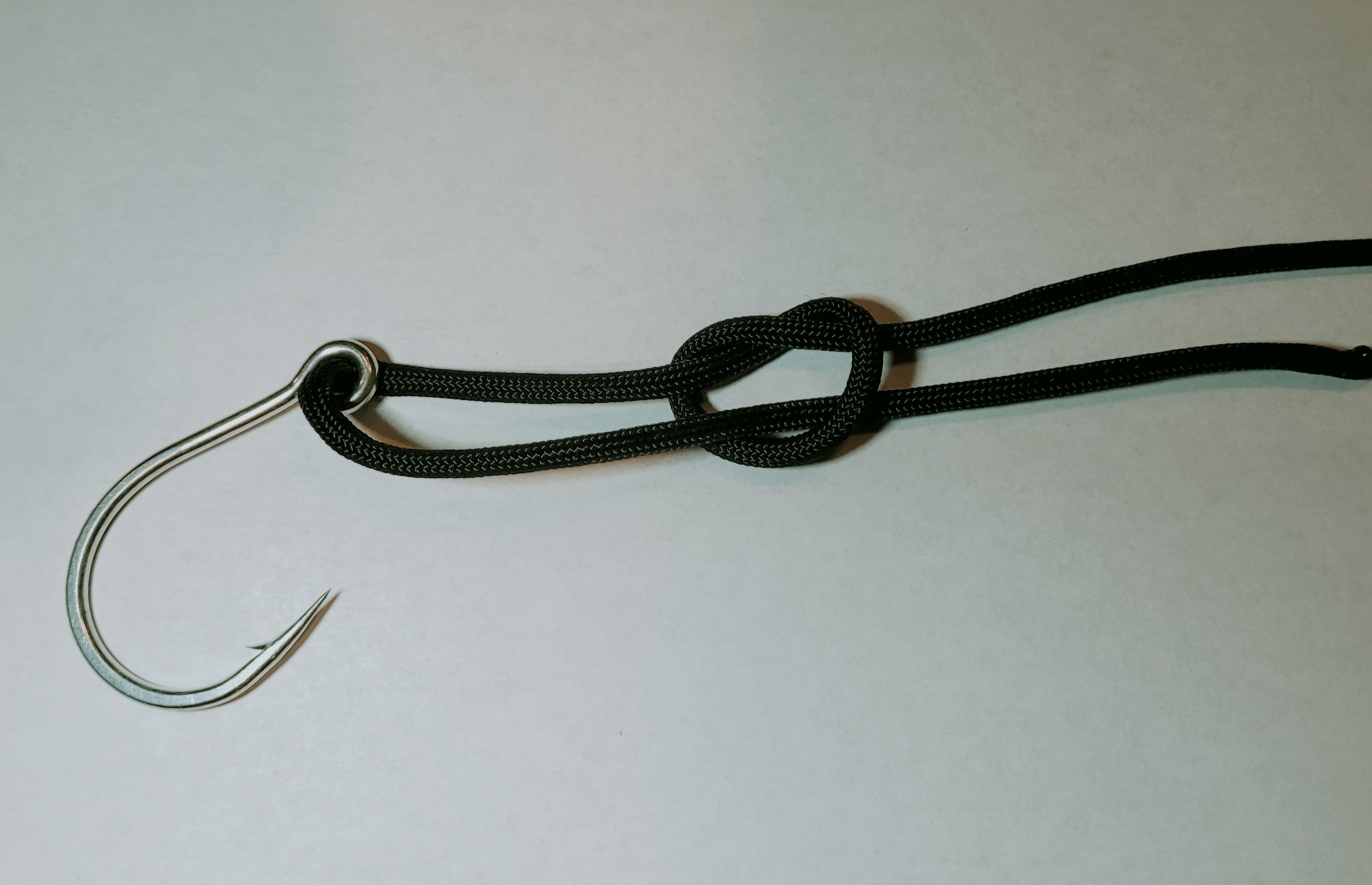
Step 2
Take the tag end of the line and run it through the eye of the hook. Then take the tag end and run it back along the line and through the overhand knot, you already tied.
Step 3
Take the tag end of the line you have through the overhand knot and then wrap it around the mainline above the overhand knot. You want at least 4 wraps, adjust the wrap count to match the line thickness. The thicker your line the fewer wraps you’ll need and vice versa.
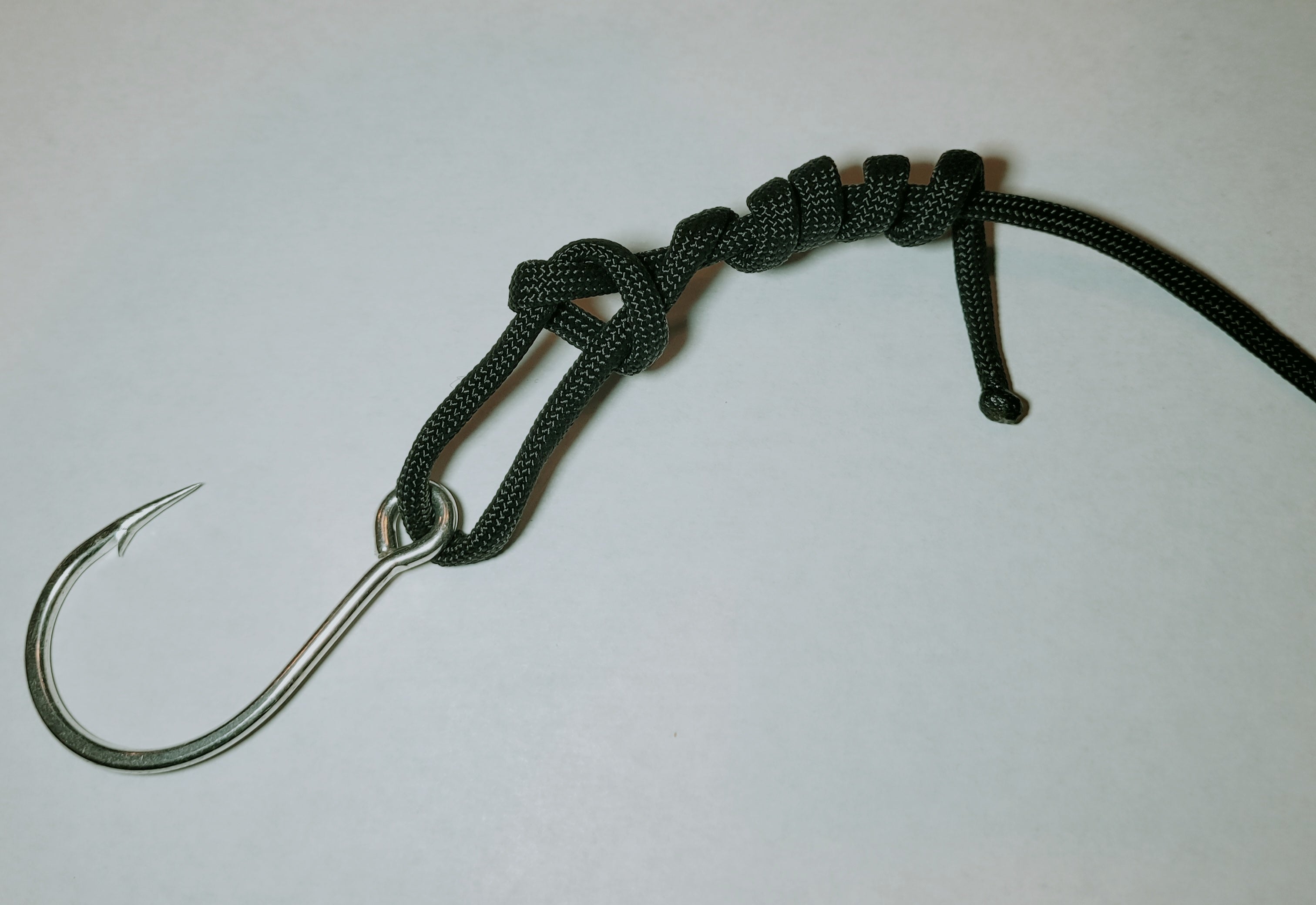
Step 4
After completing all the wraps around the mainline, take the tag end back through the overhand knot. Make sure your wraps stay tight and neat, you don’t want them overlapping each other.
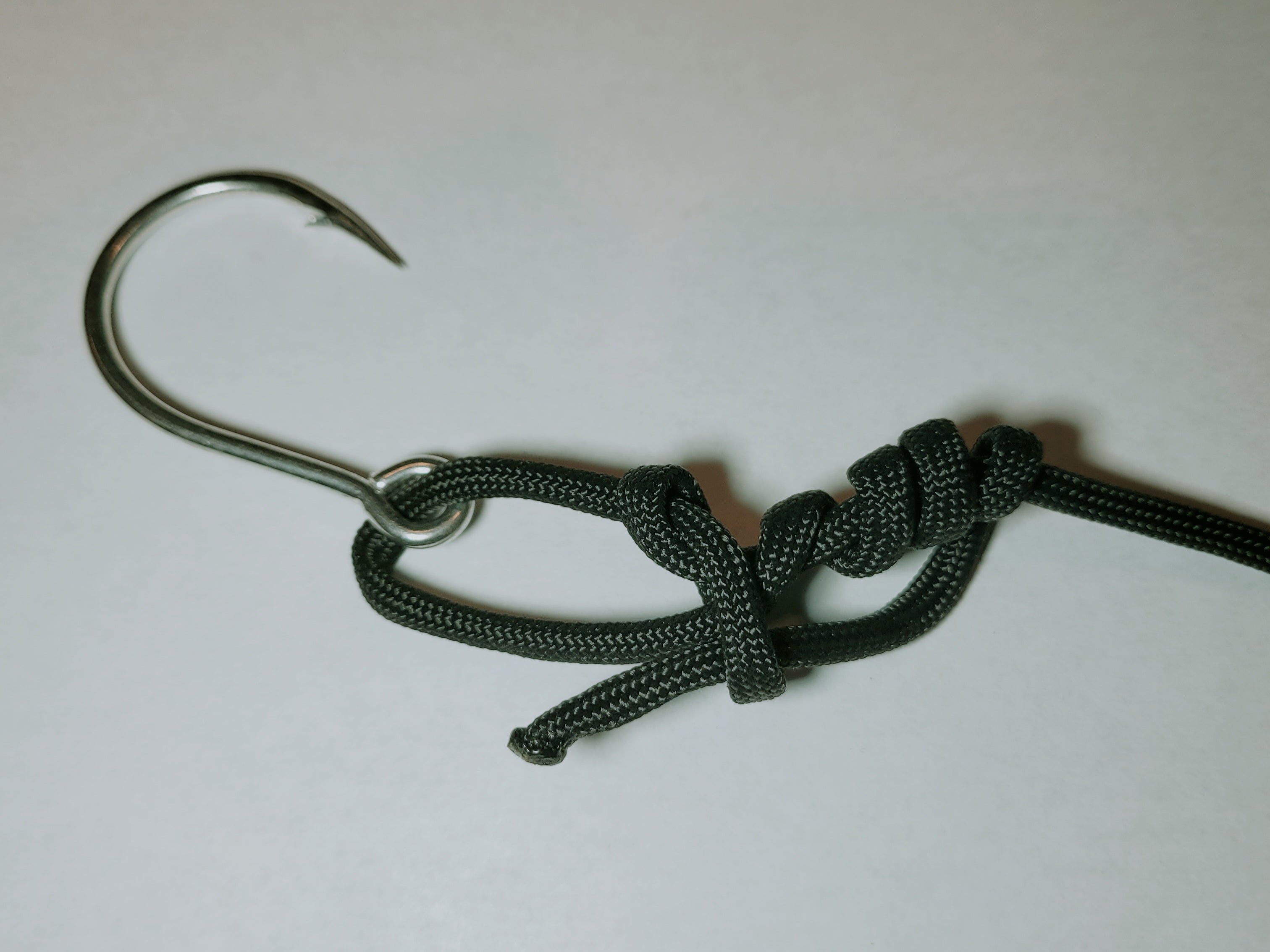
Step 5
Start tightening down the knot, pulling on the mainline and tag end. Make sure to wet the knots to avoid damaging the knot, and also make sure to adjust the loop to the size you want. This is the last chance you will have to do adjustments. Once the Non-Slip Loop Knot is exactly how you want it and tight, cut the tag close and your knot is done.
The post Are You Nuts? Know your Fishing Knots! – The Non-Slip Loop Knot appeared first on AllOutdoor.com.
AllOutdoor.com
Laravel Splade introduction video: the magic of Inertia.js with the simplicity of Blade
http://img.youtube.com/vi/9V9BUHtvwXI/0.jpgSplade provides a super easy way to build Single Page Applications (SPA) using standard Laravel Blade templates, enhanced with renderless Vue 3 components. In essence, you can write your app using the simplicity of Blade, and besides that magic SPA-feeling, you can sparkle it to make it interactive. All without ever leaving Blade.Laravel News Links
Containerizing Laravel Applications
Few technologies have gained the kind of widespread adoption that containers have. Today, every major programming language, operating system, tool, cloud provider, continuous integration (CI), and continuous deployment or delivery (CD) platform has native support for containers.
The popularity of containers has been largely driven by ground-up adoption by developers and operations teams who have seen the benefits first-hand.
In this post we’ll learn how to containerize an existing Laravel application, and along the way, we’ll explore some of the benefits that containers can bring to a developer’s workflows.
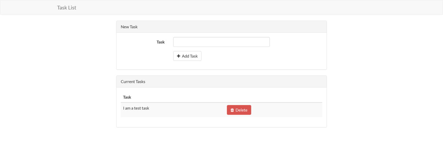
The Sample Application
For this blog post, we will containerize the sample Laravel task-list application provided on GitHub. This project was written against a reasonably old version of Laravel and has since been archived. However, working with this codebase requires that we address a number of requirements commonly found in production and legacy code bases, such as using specific versions of PHP, database migrations, port mappings, and running integration tests.
The final version of the sample application looks like this:
Prerequisites
To follow along with this blog post, you must have Docker installed on your local machine.
Windows and macOS users can find downloads and installation instructions on the Docker website.
Docker also provides packages for many Linux distributions.
Note that Windows recently began providing native support for containers. This allows native Windows software to be run inside a container. However, this post assumes that Windows developers are running Docker Desktop with Linux containers. The following PowerShell command ensures that Docker for Windows is set to work with Linux containers:
& "C:\Program Files\Docker\Docker\DockerCli.exe" -SwitchLinuxEngine
Since the application source code is stored on GitHub, the git command line (CLI) tool must also be installed. The git documentation provides installation instructions.
To run the application outside of a container, PHP 7 must be installed. The PHP website provides downloads for PHP 7.
We also need Composer to install the dependencies. The Composer documentation provides instructions on downloading and installing the tool.
Note the application won’t run on PHP 8 due to the specific version requirements defined in the composer.json file. If you try to bypass this requirement with the command composer install --ignore-platform-reqs, the following error is displayed:
Uncaught ErrorException: Method ReflectionParameter::getClass() is deprecated
The deprecation of this method is documented here. While there are options available for replacing these deprecated methods if you are willing to update the source code, we’ll treat this as an opportunity to leverage containers to resolve specific dependencies.
Cloning the Application Source Code
To clone the git repository to your local workstation, run the following command:
git clone https://github.com/laravel/quickstart-basic quickstart
This will create a directory called quickstart containing the application source code.
Running the Application Outside of a Container
To run the application outside of a container, we first need to install the dependencies:
Next, the database must be initialized. The sample application has support for a number of databases, including popular open-source projects, such as MySQL and PostgreSQL. The default is set to MySQL, so we’ll use it for this post.
Notice that we didn’t list MySQL in the prerequisites section. This is because we will run MySQL in a container, which allows us to download, configure, and run MySQL with a single docker command.
The following Bash command runs MySQL as a Docker container:
docker run --name mysql \
  -d \
  -p 3306:3306 \
  -e MYSQL_RANDOM_ROOT_PASSWORD=true \
  -e MYSQL_DATABASE=laravel \
  -e MYSQL_USER=laravel \
  -e MYSQL_PASSWORD=Password01! \
  mysql
Here is the same command for PowerShell:
docker run --name mysql `
  -d `
  -p 3306:3306 `
  -e MYSQL_RANDOM_ROOT_PASSWORD=true `
  -e MYSQL_DATABASE=laravel `
  -e MYSQL_USER=laravel `
  -e MYSQL_PASSWORD=Password01! `
  mysql
This command is doing a lot of work, so let’s break it down.
The run argument instructs Docker to run the Docker image passed as the final argument, which is mysql. As we noted in the introduction, every major tool provides a supported Docker image, and MySQL is no exception. The MySQL image has been sourced from the default Docker registry called DockerHub, which provides the repository mysql.
We define the name of the Docker container with the arguments --name mysql. If we do not specify a name, Docker will randomly assign a (often humorous) name, such as modest_shaw or nervous_goldwasser.
The -d argument runs the container in the background.
Ports to be exposed by the container are defined with the -p argument. Here, we expose the local port 3306 to the container port 3306.
Environment variables are defined with the -e argument. We have set the MYSQL_RANDOM_ROOT_PASSWORD, MYSQL_DATABASE, MYSQL_USER, and MYSQL_PASSWORD environment variables to configure MySQL with a random root password, an initial database called laravel, a user account called laravel, and the user password of Password01!.
The final argument mysql is the name of the Docker image used to create the container.
The ability to download and run tools, as we have done with MySQL, is one of the major benefits of Docker and containers. Whereas installing the specific versions of PHP and Composer noted in the prerequisites section requires visiting multiple web pages to download specific packages or run unique installation commands, the command to run a Docker image is the same for every operating system and every tag of a Docker image.
A lot of Docker-specific terms, such as registry, repository, image and container, were used to describe the command above. We’ll cover these terms in later sections, but for now, we’ll move on to running our sample application locally.
To initialize the database, we first set a number of environment variables read by the application to connect to the database. You’ll notice that these values match those used when running MySQL as a container.
The following commands set the environment variables in Bash:
export DB_HOST=localhost
export DB_DATABASE=laravel
export DB_USERNAME=laravel
export DB_PASSWORD=Password01!
These are the equivalent PowerShell commands:
$env:DB_HOST="localhost"
$env:DB_DATABASE="laravel"
$env:DB_USERNAME="laravel"
$env:DB_PASSWORD="Password01!"
We then run the database migration with the following command:
Tests are run with the following command:
Finally, we run the sample application, hosted by a development web server, with the following command:
We can then open http://localhost:8000 to view the task list.
Even though we used Docker to download and run MySQL with a single command, a lot of tools needed to be installed. Some of these tools required specific versions, usually with slightly different processes between operating systems, and many individual commands had to be executed to reach the point of running this simple application.
Docker can help us here by allowing us to compile, test, and run our code with a small number of calls to docker. As we have seen, we can also run other applications like MySQL with docker commands. Best of all, the commands are the same for every operating system.
Before we continue, though, lets dig into some of the Docker terms used above in more detail.
Docker Registry and Repository
A Docker registry is much like the online collection of packages used by Linux package managers, such as apt or yum, Windows package managers like Chocolatey, or macOS package managers like Brew. A Docker registry is a collection of Docker repositories, where each Docker repository provides many versions (or tags in Docker terminology) of a Docker image.
Docker Image and Container
A Docker image is a package containing all the files required to run an application. This includes the application code (e.g., the Laravel sample application), runtime (e.g., PHP), system libraries (e.g., the dependencies PHP relies on), system tools (e.g., web servers like Apache), and system settings (e.g., network configuration).
A container is an isolated environment in which the image is executed. While containers cannot traditionally be relied on to enforce the kind of isolation provided by a virtual machine (VM), they are routinely used to execute trusted code side-by-side on a single physical or virtual machine.
A container has its own isolated network stack. This means that by default, code running in one Docker container cannot interact over the network with another docker container. To expose a container to network traffic, we need to map a host port to a container port. This is what we achieved with the -p 3306:3306 argument, which mapped port 3306 on the host to port 3306 on the container. With this argument, traffic to localhost on port 3306 is redirected to port 3306 in the container.
Creating a Basic PHP Docker Image
We have seen the commands that must be run directly on our workstation to build and run the Laravel application. Conceptually, building a Docker image involves scripting those same commands in a file called Dockerfile.
In addition to running commands to download dependencies and execute tests, a Dockerfile also contains commands to copy files from the host machine into the Docker image, expose network ports, set environment variables, set the working directory, define the command to be run by default when a container is started, and more. The complete list of instructions can be found in the Docker documentation.
Let’s look at a simple example. Save the following text to a file called Dockerfile somewhere convenient on your local workstation:
FROM php:8
RUN echo "<?php\n"\
    "print 'Hello World!';\n"\
    "?>" > /opt/hello.php
CMD ["php", "/opt/hello.php"]
The FROM instruction defines the base image that our image will build on top of. We take advantage of the fact that all major programming languages provide officially supported Docker images that include the required runtime, and in this example, we’ve used the php image from DockerHub. The colon separates the image name from the tag, and the 8 indicates the tag, or version, of the image to use:
The RUN instruction executes a command within the context of the image being created. Here, we echo a simple PHP script that prints Hello World! to the file /opt/hello.php. This creates a new file within our Docker image:
RUN echo "<?php\n"\
    "print 'Hello World!';\n"\
    "?>" > /opt/hello.php
The CMD instruction configures the command to be run when a container based on this image is run. Here, we use an array to build up the components of the command, starting with a call to php and then passing it the file we created with the previous RUN instruction:
CMD ["php", "/opt/hello.php"]
Build an image with the command:
docker build . -t phphelloworld
The docker build command is used to build new Docker images. The period indicates that the Dockerfile is in the current working directory. The -t phphelloworld argument defines the name of the new image.
Then, create a container based on the image with the following command:
You will see Hello World! printed to the console as PHP executes the script saved to /opt/hello.php.
Creating a Docker image from an existing PHP application follows much the same process as this simple example. The application source code files are copied into the Docker image instead of creating them with echo commands. Some additional tooling is installed to allow the dependencies to be downloaded, and additional PHP modules are installed to support the build process and database access, but fundamentally, we use the same set of instructions to achieve the required outcome.
Let’s look at how we can containerize the sample Laravel application.
Containerizing the Laravel application
As we saw with the example above, we can run almost any command we want in the process of building a Docker image.
As part of the process of building the application, we need to download dependencies, and we’ll also run any tests to ensure the code being built is valid. The tests included in this application require access to an initialized database, which we must accommodate as part of the image build process.
Running the application also requires access to a database, and we can’t assume the database that was used for the tests is also the same database used to run the application. So, before the application is run, we’ll need to run the database migrations again to ensure our application has the required data.
Let’s look at a Dockerfile that downloads dependencies, initializes the test database, runs tests, configures the database the application is eventually run against, and then launches the application, all while ensuring the required version of PHP is used.
Writing the Dockerfile
Here is an example of a Dockerfile saved in the quickstart directory that the sample application code was checked out to:
FROM php:7
ENV PORT=8000
RUN apt-get update; apt-get install -y wget libzip-dev
RUN docker-php-ext-install zip pdo_mysql
RUN wget https://raw.githubusercontent.com/composer/getcomposer.org/master/web/installer -O - -q | php -- --install-dir=/usr/local/bin --filename=composer
WORKDIR /app
COPY . /app
RUN composer install
RUN touch /app/database/database.sqlite
RUN DB_CONNECTION=sqlite php artisan migrate
RUN DB_CONNECTION=sqlite vendor/bin/phpunit
RUN echo "#!/bin/sh\n" \
  "php artisan migrate\n" \
  "php artisan serve --host 0.0.0.0 --port \$PORT" > /app/start.sh
RUN chmod +x /app/start.sh
CMD ["/app/start.sh"]
Let’s break this file down.
As with the previous “Hello World!” example, we based this Docker image on the php image. However, this time, we use the tag 7 to ensure the base image has PHP 7 installed. If you recall, we must use PHP 7 due to methods used by this sample application that were deprecated in PHP 8.
It is worth taking a moment to appreciate how simple Docker makes it to build and run applications with different versions of PHP side-by-side on a single machine.
At a minimum, to run multiple versions of PHP without Docker, you would have to download PHP 7 and 8 to different directories and remember to call the appropriate executable between projects. Your operating system’s package manager may offer the ability to install multiple versions of PHP, but the process for doing so would differ between Linux, macOS, and Windows.
With Docker, the ability to match a specific PHP version to the code being run is an inherent feature because each Docker image is a self-contained package with all the files required to run an application:
The ENV instruction defines an environment variable. Here, we define a variable called PORT and give it a default value of 8000. We’ll use this variable when launching the web server:
The php base image is based on Debian, which means we use apt-get for package management. Here, we update the list of dependencies with apt-get update, and then install wget and the zip development libraries:
RUN apt-get update; apt-get install -y wget libzip-dev
Our Laravel application requires the zip and pdo_mysql PHP extensions to build and run. The php base image includes a helper tool called docker-php-ext-install that installs PHP extensions for us:
RUN docker-php-ext-install zip pdo_mysql
To build the application, we need Composer to download the dependencies. Here, we download the Composer installation script with wget and execute it to install Composer to /usr/local/bin/composer:
RUN wget https://raw.githubusercontent.com/composer/getcomposer.org/master/web/installer -O - -q | php -- --install-dir=/usr/local/bin --filename=composer
The WORKDIR instruction sets the working directory for any subsequent commands, such as RUN or CMD. Here, we set the working directory to a new directory called /app:
The COPY instruction copies files from the host machine into the Docker image. Here, we copy all the files from the current directory into the directory called /app inside the Docker image:
Here, we install the application dependencies with composer:
The tests require access to a database to complete. For convenience, we will use SQLite, which is a local in-memory database that requires a file to be created to host the database table:
RUN touch /app/database/database.sqlite
Because the tests in the project require an initialized database, we configure the migration script to use SQLite and run php artisan migrate to create an required tables:
RUN DB_CONNECTION=sqlite php artisan migrate
We then run any tests included in the code. If these tests fail, the operation to build the Docker image will also fail, ensuring we only build an image if the tests pass successfully:
RUN DB_CONNECTION=sqlite vendor/bin/phpunit
If we have reached this point, the tests have passed, and we now configure the image to run the Laravel application when the container starts. The echo command here writes a script to /app/start.sh. The first command in the script runs the database migration, and the second launches the development web server. The command php artisan serve --host 0.0.0.0 --port=$PORT ensures that the web server listens to all available IP addresses, which is required for Docker to map a port on the host into the container and listen on the port defined in the environment variable PORT:
RUN echo "#!/bin/sh\n" \
  "php artisan migrate\n" \
  "php artisan serve --host 0.0.0.0 --port \$PORT" > /app/start.sh
The script file we just created needs to be marked as executable to run:
RUN chmod +x /app/start.sh
The final instruction defines the command to be run when a container based on this image is started. We launch the script created above to initialize the database and start the web server:
Before we build the image, we need to create a file called .dockerignore alongside Dockerfile with the following contents:
The .dockerignore file lists the files and directories that will be excluded from instructions like COPY . /app. Here, we have instructed Docker to ignore any files that may have been downloaded by a call to composer install on the host machine. This ensures that all the dependencies are freshly downloaded as the Docker image is built.
We can now build the Docker image with the following command:
docker build . -t laravelapp
We can then watch as Docker executes the instructions defined in the Dockerfile to copy and build the sample application.
Assuming that you still have the MySQL Docker container running, run the Laravel image with the following command. Note that the database host is set to host.docker.internal. This is a special hostname exposed by Docker in a container on Windows and macOS hosts that resolves to the host. This allows code running in a container to interact with services running on the host machine:
docker run -p 8001:8000 -e DB_HOST=host.docker.internal -e DB_DATABASE=laravel -e DB_USERNAME=laravel -e DB_PASSWORD=Password01! laravelapp
Linux users do not have access to the host.docker.internal hostname and must instead use the IP address of 172.17.0.1:
docker run -p 8001:8000 -e DB_HOST=172.17.0.1 -e DB_DATABASE=laravel -e DB_USERNAME=laravel -e DB_PASSWORD=Password01! laravelapp
To understand where the IP address of 172.17.0.1 comes from, run the following command:
docker network inspect bridge
This will display technical information about the bridge network, which is the default network we have been running the Docker containers in. The output below has been stripped down to show the important value of Gateway, which defines the IP address a container can connect to reach the host. As you can see, this is where 172.17.0.1 comes from:
[
    {
        "IPAM": {
            "Config": [
                {
                    "Gateway": "172.17.0.1"
                    ...
                }
                ...
            ]
        },
        ...
    }
]
We have used -p 8001:8000 to map port 8001 on the host to port 8000 in the container. We then set a number of environment variables to configure the Laravel application to use the MySQL Docker container.
Open http://localhost:8001 to access the sample application running inside a Docker container.
We now have a self-contained Docker image that can be distributed to other developers or platforms that host Docker containers. However, the image we just created only exists on our local workstation. In the next section, we’ll configure a CI pipeline to build this image automatically and publish it to a Docker repository.
Creating a CI Pipeline
There are any number of CI platforms that can be used to build Docker images. For this post, we’ll make use of GitHub Actions.
GitHub Actions is a service built into GitHub, and it provides an execution environment and plugin ecosystem that allows us to easily automate common tasks, such as building Docker images.
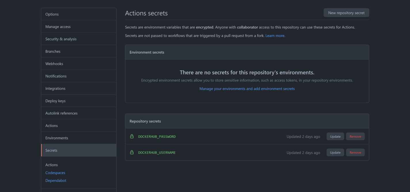
We will publish the final image to a Docker repository called DockerHub. You can sign up for a free account here. The free account allows you to publish public Docker images to be shared with anyone, making it a convenient option for open-source applications.
We need to capture our DockerHub credentials as secrets in GitHub. This is done by opening Settings -> Secrets in the GitHub repository. We need to create two secrets: DOCKERHUB_USERNAME, containing our DockerHub username, and DOCKERHUB_PASSWORD, containing our DockerHub password:
The CI pipeline is defined in a file called .github/workflows/main.yaml. The complete code is shown below:
name: CI

on:
  push:

jobs:
  build:
    runs-on: ubuntu-latest
    steps:
      - uses: actions/checkout@v2

      - name: Set up Docker Buildx
        uses: docker/setup-buildx-action@v1

      - name: Login to DockerHub
        uses: docker/login-action@v1
        with:
          username: $
          password: $

      - name: Build and push
        id: docker_build
        uses: docker/build-push-action@v2
        with:
          push: true
          tags: $/laravelapp
          build-args: |
            db_host=172.17.0.1
            db_username=laravel
            db_database=laravel
            db_password=Password01!
The name property defines the name of the workflow:
The on property defines when the workflow is triggered. The child push property configures this workflow to run each time a change is pushed to the git repository:
The jobs property is where one or more named processes are defined. The build property creates a job of the same name:
The build job will be run on an Ubuntu VM:
Each job consists of a number of steps that combine to achieve a common outcome, which, in our case, is to build and publish the Docker image:
The first step is to checkout the git repository:
- uses: actions/checkout@v2
We then use the docker/setup-buildx-action action to initialize an environment to build Docker images:
      - name: Set up Docker Buildx
        uses: docker/setup-buildx-action@v1
The credentials we configured earlier are used to log into DockerHub:
      - name: Login to DockerHub
        uses: docker/login-action@v1
        with:
          username: $
          password: $
Finally, we use the docker/build-push-action action to build the Docker image. By setting the with.push property to true, the resulting image will be pushed to DockerHub.
Note that the with.tags property is set to $/laravelapp, which will resolve to something like mcasperson/laravelapp (where mcasperson is my DockerHub username). Prefixing the image name with a username indicates the Docker registry that the image will be pushed to. You can see this image pushed to my DockerHub account here:
      - name: Build and push
        id: docker_build
        uses: docker/build-push-action@v2
        with:
          push: true
          tags: $/laravelapp
With this workflow defined in GitHub, each commit to the git repository will trigger the Docker image to be rebuilt and published, giving us a CI pipeline.
The published image can be run with the following command. Replace mcasperson with your own DockerHub username to pull the image from your own public repository.
Here is the Bash command:
docker run \
  -p 8001:8000 \
  -e DB_HOST=172.17.0.1 \
  -e DB_DATABASE=laravel \
  -e DB_USERNAME=laravel \
  -e DB_PASSWORD=Password01! \
  mcasperson/laravelapp
Here is the equivalent PowerShell command:
docker run `
  -p 8001:8000 `
  -e DB_HOST=172.17.0.1 `
  -e DB_DATABASE=laravel `
  -e DB_USERNAME=laravel `
  -e DB_PASSWORD=Password01! `
  mcasperson/laravelapp
You can find a fork of the sample application repository that contains the GitHub Actions workflow above here.
Deploying the Container
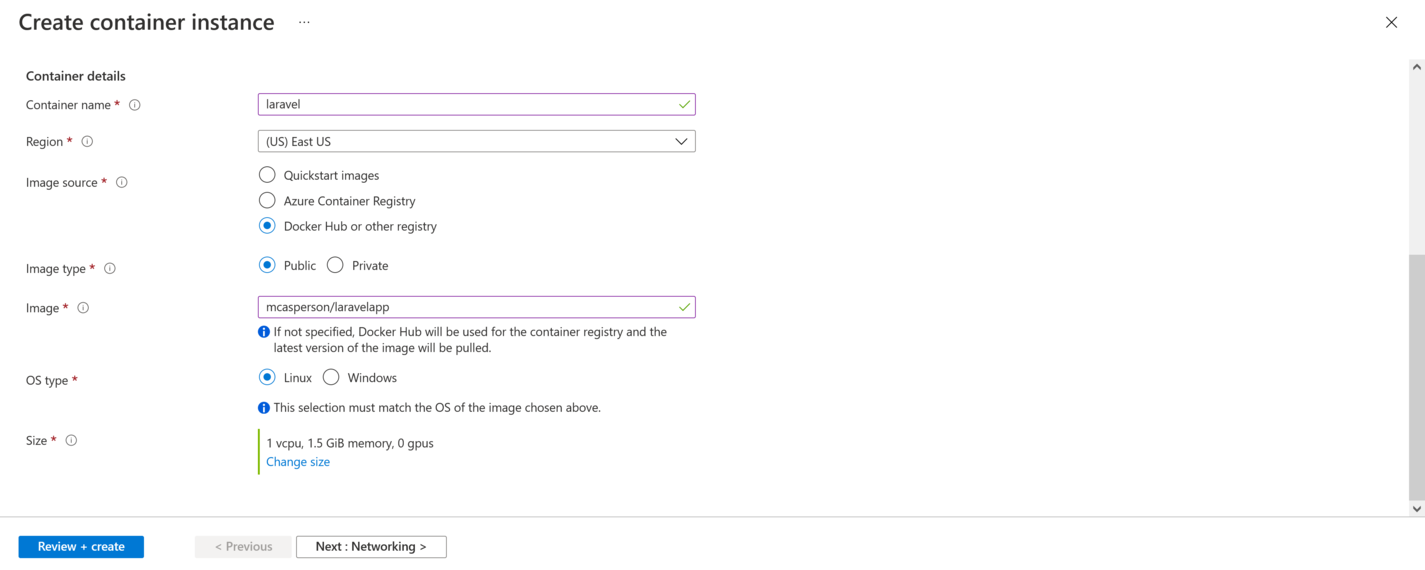
If there is one benefit to containerizing your applications, it is the incredible range of platforms that they can be deployed to. You can deploy containers to Kubernetes or any of the managed Kubernetes platforms, such as Azure Kubernetes Service (AKS), AWS Elastic Kubernetes Service (EKS), or Google Kubernetes Engine (GKE). Azure also has Container Instances, while AWS has App Runner, and Google has Cloud Run.
In addition to the major cloud providers, you can deploy containers to Heroku, Dokku, Netlify, and many more.
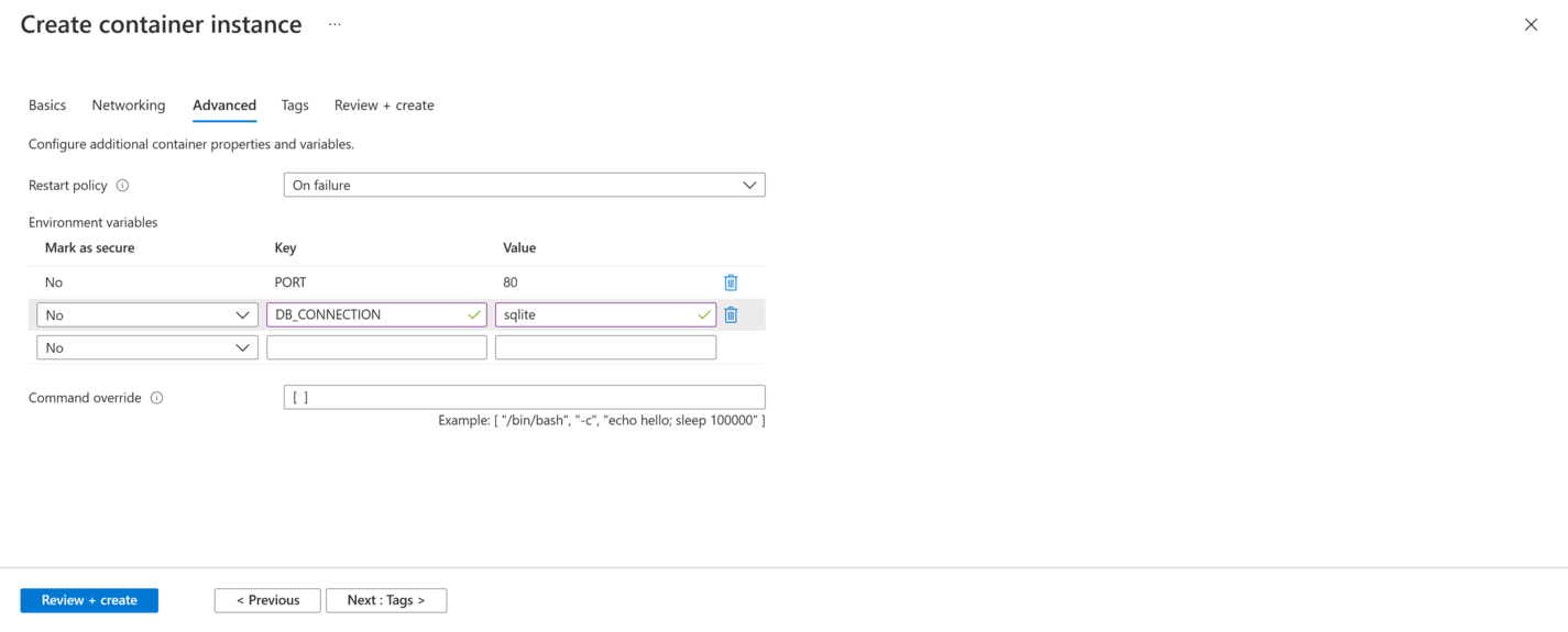
In the screenshots below, I have deployed the image to an Azure Container Instance. It involves pointing the container instance to the public Docker image and setting a few environment variables to configure the port and database settings. With a few clicks, the application is deployed and publicly accessible:
Conclusion
In this post, we presented a process to containerize Laravel PHP applications. By containerizing an old sample application created by the Laravel project, we encountered many real-world concerns, including PHP version dependencies, PHP extensions, integration tests requiring database access, database migration scripts, and initializing supporting infrastructure like MySQL databases.
We also presented a process for continuous integration with a sample GitHub Actions workflow to build and publish the resulting Docker image and saw how the image could be deployed to one of the many hosting platforms that support Docker.
The end result allows us to build and test our Laravel application with one simple call to docker, which, in turn, generates a Docker image that anyone can download and run with one or two additional docker calls. This makes it much easier for developers to consume the project and for operations staff to deploy.
Honeybadger has your back when it counts.
We combine error tracking, uptime monitoring, and cron & heartbeat monitoring into a simple, easy-to-use platform. Our mission: to tame production and make you a better, more productive developer.
Laravel News Links
Watch: Weatherman goes viral for ‘accidentally’ drawing a weiner to show Hurricane Ian pounding Florida
https://www.louderwithcrowder.com/media-library/image.png?id=31842184&width=980
Florida is the most phallic looking of all the states. You can’t mistake the angle of the dangle. Knowing his state’s similarity to what used to be known exclusively as male genitalia (pre-2021), you would think an experienced weatherman like Bryan Norcross would be more careful with his telecaster. Or, maybe this is his way of illustrating how Hurricane Ian was going to f*ck Florida hard.
Whatever the reason, he’s going viral for the following unfortunate illustration.
This guy has been doing this ALL DAY LONG#HurricaneIan pic.twitter.com/odd0kgzUHp
— ALT-immigration (@ALT_uscis) September 26, 2022
Dude.
Penis Song – Monty Python’s The Meaning of Life
youtu.be
I put "accidentally" in quotes because I’m of the belief when something that looks like a cock gets drawn on a map or a news graphic, the dude drawing knows what they’re doing. It’s like what Jim Halbert taught us on The Office. If there’s an opportunity for someone to work in a phallic shape, interacting with the artwork (or in this case, a hurricane map), it’ll happen
Apparently, our guy is a local celebrity.
Bryan Norcross was the weather guy who got us through Hurricane Andrew 30 years ago. Now with Fox weather, he’s drawing Ian dick on the tv #signothetimes pic.twitter.com/AtUQEnJoMa
— Nicole Sandler (@nicolesandler) September 28, 2022
I’m a simple man. I like cold beer, loud music, and taking every available opportunity for a euphamism. That may not have been Norcross’ intent. But it was the intent of an easily amused internet.
I didn’t know Fox had a weather channel and there’s some interesting stuff going on there 🤣🍆 pic.twitter.com/SDWCOVYz5A
— Wu-Tang Is For The Children (@WUTangKids) September 27, 2022
“And now let’s go to Bryan Norcross with the weather foresk— sorry -cast!” https://t.co/bcCIMIHL55
— Craig Winneker (@CraigWinneker) September 27, 2022
Bryan Norcross let everyone know Hurricane Ian is screwing Florida pic.twitter.com/GKTnRKGFxF
— Brucito (@BartonTheBruce) September 27, 2022
Anyone who has been in a hurricane before knows, as long you are not in danger, you pass the time amusing yourselves however possible. Florida has been proving that over the past forty-eight hours. Maybe it was a coincidence the way Hurricane Ian was traveling required drawing two circles and a giant line ending at the tip where the hurricane symbol was. Or maybe after thirty years of covering hurricanes, Bryan Norcross felt some childish humor was in order. Either way, Hurricane Ian is being a dick.
Facebook doesn’t want you reading this post or any others lately. Their algorithm hides our stories and shenanigans as best it can. The best way to stick it to Zuckerface? Bookmark LouderWithCrowder.com and check us out throughout the day!
Also follow us on Instagram, Twitter and Gettr!
Psycho Uses THIS EXCUSE to Skip the Walmart Line | Louder With Crowder
youtu.be
Louder With Crowder
Give Me Some Latitude… and Longitude
https://www.percona.com/blog/wp-content/uploads/2022/09/Geo-locations-in-MySQL.png
 Geo locations are a cornerstone of modern applications. Whether you’re a food delivery business or a family photographer, knowing the closest “something” to you or your clients can be a great feature.
In our ‘Scaling and Optimization’ training class for MySQL, one of the things we discuss is column types. The spatial types are only mentioned in passing, as less than 0.5% of MySQL users know of their existence (that’s a wild guess, with no factual basis). In this post, we briefly discuss the POINT type and how it can be used to calculate distances to the closest public park.
Import the data
To start off, we need a few tables and some data. The first table will hold the mapping between the zip code and its associated latitude/longitude. GeoNames has this data under the Creative Commons v3 license, available here for most countries. The data files are CSV and the readme.txt explains the various columns. We are only interested in a few of the columns.
CREATE TABLE usazips (
 id int unsigned NOT NULL AUTO_INCREMENT,
 zipCode int unsigned NOT NULL COMMENT 'All USA postal codes are integers',
 state varchar(20) NOT NULL,
 placeName varchar(200) NOT NULL,
 placeDesc varchar(100) DEFAULT NULL,
 latLong point NOT NULL /*!80003 SRID 4326 */,
 PRIMARY KEY (id));
There are a couple of things about this schema that are not typical in MySQL.
Firstly, the latLong column type is POINT which can store an X and Y coordinate. By default, these coordinates could be on any plane. They could represent latitude and longitude, but they could also be centimeters up and down on the surface of your desk, or yards left and right of the biggest tree at your local park. How do you know which? You need a Spatial Reference System. Thankfully, MySQL comes preloaded with about 5,100 of these systems (See INFORMATION_SCHEMA.ST_SPATIAL_REFERENCE_SYSTEMS). Each SRS has an associated Spatial Reference ID (SRID).
The SQL comment on the POINT column above ties the data in this column with a specific SRID, 4326. We can see in the I_S table noted earlier, this SRID maps to the ‘World Geodetic System 1984’ (aka WGS84) which is the same SRS used in the GeoNames dataset. By having our column and the dataset aligned, we won’t need to do any geo-transformation later on.
The second thing to note in the schema is the use of a SPATIAL index on the latLong column. A SPATIAL index in MySQL is created using R-Trees which are geospatial-specific data structures.
Let’s load this data into the table. There are 12 fields in the CSV but we only care about six of them. The LOAD DATA command allows you to associate each CSV field, positionally, with either the column name in the table or a user variable. The first field in our CSV is the country code, which we don’t care about, so we assign that field to the @dummy variable. The second field is the zip code, and we want that to go directly into the table-column so we specify the column name. We do the same for the third, fifth, sixth, and ninth fields.
The 10th and 11th CSV fields are the latitude and longitude. We need to convert those two VARCHAR fields into a POINT. We can apply some SQL transformations using the SET command which can reference user variables assigned earlier. These two fields are assigned to @lat and @lon. The remaining fields all go into @dummy since they are not used.
LOAD DATA INFILE '/var/lib/mysql-files/US.txt'
INTO TABLE usazips
FIELDS TERMINATED BY '\t' (@dummy, zipCode, placeName, @dummy, state, placeDesc, @dummy, @dummy, @dummy, @lat, @lon, @dummy)
SET id = NULL, latLong = ST_PointFromText(CONCAT('POINT(', @lat, ' ', @lon, ')'), 4326);
Unfortunately, the POINT() function in MySQL always returns an SRID of 0. Since we specified our column to be a specific SRID, a direct import will fail.
mysql> LOAD ... SET latLong = POINT(@lat, @lon);
ERROR 3643 (HY000): The SRID of the geometry does not match the SRID of the column 'latLong'.
The SRID of the geometry is 0, but the SRID of the column is 4326. Consider changing the SRID
of the geometry or the SRID property of the column.
Instead, we must “go the long route” by creating a string representation of a POINT object in the Well-Known-Text format, which MySQL can parse into a Point column type with an associated SRID.
mysql> LOAD ... SET latLong = ST_PointFromText(CONCAT('POINT(', @lat, ' ', @lon, ')'), 4326);
Yes, this was very confusing to me as well:
“POINT(123 56)” <— WKT Format (a string)
POINT(123, 56) <— MySQL Column Type (function that returns data)
Here’s a quick verification of our data with an additional column showing the lat-long binary data being converted back into WKT format.
mysql> SELECT *, ST_AsText(latLong) FROM usazips WHERE zipCode = 76455;
+-------+---------+-------+-----------+-----------+------------------------------------------------------+-------------------------+
| id    | zipCode | state | placeName | placeDesc | latLong                                              | ST_AsText(latLong)      |
+-------+---------+-------+-----------+-----------+------------------------------------------------------+-------------------------+
| 34292 |   76455 | TX    | Gustine   | Comanche  | 0xE6100000010100000068B3EA73B59958C0B84082E2C7D83F40 | POINT(31.8468 -98.4017) |
+-------+---------+-------+-----------+-----------+------------------------------------------------------+-------------------------+
1 row in set (0.04 sec)
More data to load
Now that we have all this zip code + latitude and longitude data, we next need the locations of where we want to find our distances. This could be a list of grocery stores or coffee shops. In this example, we will use a list of public parks in San Antonio, TX. Thankfully, San Antonio has all of this data openly available. I downloaded the ‘Park Boundaries’ dataset in GeoJSON format since the CSV did not contain any latitude/longitude coordinates.
CREATE TABLE parks (
 parkId int unsigned NOT NULL PRIMARY KEY,
 parkName varchar(100) NOT NULL,
 parkLocation point NOT NULL /*!80003 SRID 4326 */);
The GeoJSON data is one giant JSON string with all of the needed data nested in various JSON objects and arrays. Instead of writing some Python script to ETL the data, I decided to try out the JSON import feature of the MySQL Shell and first import the JSON directly into a temporary table.
$ mysqlsh appUser@127.0.0.1/world --import Park_Boundaries.geojson tempParks
Importing from file "Park_Boundaries.geojson" to collection `world`.`tempParks` in MySQL Server at 127.0.0.1:33060
..1..1
Processed 3.29 MB in 1 document in 0.3478 sec (1.00 document/s)
Total successfully imported documents 1 (1.00 document/s)
The MySQL Shell utility created a new table called ‘tempParks’, in the ‘world’ database with the following schema. One row was inserted, which was the entire dataset as one JSON object.
CREATE TABLE `tempParks` (
 `doc` json DEFAULT NULL,
 `_id` varbinary(32) GENERATED ALWAYS AS (json_unquote(json_extract(`doc`,_utf8mb4'$._id'))) STORED NOT NULL,
 `_json_schema` json GENERATED ALWAYS AS (_utf8mb4'{"type":"object"}') VIRTUAL,
 PRIMARY KEY (`_id`),
 CONSTRAINT `$val_strict_75A2A431C77036365C11677C92B55F4B307FB335` CHECK (json_schema_valid(`_json_schema`,`doc`)) /*!80016 NOT ENFORCED */
);
From here, I extracted the needed information from within the JSON and inserted it into the final table, shown above. This SQL uses the new JSON_TABLE function in MySQL 8 to create a result set from nested JSON data (strangely, there were a couple of duplicate parks in the dataset, which is why you see the ON DUPLICATE modifier). Note: that this dataset does longitude at index 0, and latitude at index 1.
INSERT INTO parks
  SELECT k.parkID, k.parkName, ST_PointFromText(CONCAT('POINT(', parkLat, ' ', parkLon, ')'), 4326)
  FROM tempParks, JSON_TABLE(
    tempParks.doc,
    "$.features[*]" COLUMNS (
      parkID int PATH "$.properties.ParkID",
      parkName varchar(150) PATH "$.properties.ParkName",
      parkLat varchar(20) PATH "$.geometry.coordinates[0][0][0][1]",
      parkLon varchar(20) PATH "$.geometry.coordinates[0][0][0][0]"
    )
  ) AS k ON DUPLICATE KEY UPDATE parkId = k.parkID;

Query OK, 391 rows affected (0.11 sec)
Records: 392  Duplicates: 0  Warnings: 0
What’s the closest park?
Now that all the information is finally loaded, let’s find the nearest park to where you might live, based on your zip code.
First, get the reference location (as MySQL POINT data) for the zip code in question:
mysql> SELECT latLong INTO @zipLocation FROM usazips WHERE zipCode = 78218;
Then, calculate the distance between our reference zip code and all of the park locations. Show the five closest (not including any school parks):
mysql> SELECT p.parkName, ST_AsText(p.parkLocation) AS location, ST_Distance_Sphere(@zipLocation, p.parkLocation) AS metersAway
FROM parks p WHERE parkName NOT LIKE '%School%' ORDER BY metersAway LIMIT 5;
+-----------------------+----------------------------------------------+--------------------+
| parkName              | location                                     | metersAway         |
+-----------------------+----------------------------------------------+--------------------+
| Robert L B Tobin Park | POINT(29.501796110000043 -98.42111988)       |   1817.72881969296 |
| Wilshire Terrace Park | POINT(29.486397887000063 -98.41776879999996) | 1830.8541086553364 |
| James Park            | POINT(29.48168424800008 -98.41725954999998)  |  2171.268012559491 |
| Perrin Homestead Park | POINT(29.524477369000067 -98.41258342199997) |  3198.082796589456 |
| Tobin Library Park    | POINT(29.510899863000077 -98.43343147299998) |  3314.044809806559 |
+-----------------------+----------------------------------------------+--------------------+
5 rows in set (0.01 sec)
The closest park is 1,817.7 meters away! Time for a picnic!
Conclusion
Geo locations in MySQL are not difficult. The hardest part was just finding the data and ETL’ing into some tables. MySQL’s native column types and support for the OpenGIS standards make working with the data quite easy.
Several things to note:
1) The reference location for your zip code may be several hundred or a thousand meters away. Because of this, that park that is right behind your house might not show up as the actual closest because another park is closer to the reference.
2) No SPATIAL indexes were added to the tables as they would be of no use because we must execute the distance function against all parks (ie: all rows) to find the closest park, hence the ‘metersAway’ query will always perform a full table scan.
3) All USA postal codes are integers. You can expand this to your country by simply changing the column type.
Planet MySQL
MySQL: Data for Testing
https://blog.koehntopp.info/uploads/2022/09/test-data-01.jpg
Where I work, there is an ongoing discussion about test data generation.
At the moment we do not replace or change any production data for use in the test environments, and we don’t generate test data.
That is safe and legal, because production data is tokenized.
That is, PII and PCI data is being replaced by placeholder tokens which can be used by applications to access the actual protected data through specially protected access services.
Only a very limited circle of people is dealing with data in behind the protected services.
Using production data in test databases is also fast, because we copy data in parallel, at line speed, or we make redirect-on-write (“copy-on-write” in the age of SSD) writeable snapshots available.
Assume for a moment we want to change that and
- mask data from production when we copy it to test databases
- reduce the amount of data used in test databases, while maintaining referential integrity
- generate test data sets of any size instead of using production data, keeping referential integrity and also some baseline statistical properties
Masking Data
Assume we make a copy of a production database into a test setup.
We then prepare that copy by changing every data item we want to mask, for example by replacing it with sha("secret" + original value), or some other replacement token.
kris@localhost [kris]> select sha(concat("secret", "Kristian Köhntopp"));
+---------------------------------------------+
| sha(concat("secret", "Kristian Köhntopp")) |
+---------------------------------------------+
| 9697c8770a3def7475069f3be8b6f2a8e4c7ebf4 |
+---------------------------------------------+
1 row in set (0.00 sec)
Why are we using a hash function or some moral equivalent for this?
We want to keep referential integrity, of course.
So each occurence of Kristian Köhntopp will be replaced by 9697c8770a3def7475069f3be8b6f2a8e4c7ebf4, a predictable and stable value, instead of a random number 17 on the first occurence, and another random number, 25342, on the next.
In terms of database work, it means that after copying the data, we are running an update on every row, creating a binlog entry for each change.
If the column we change is indexed, the indexes that contain the column need to be updated.
If the column we change is a primary key, the physical location of the record in the table also changes, because InnoDB clusters data on primary key.
In short, while copying data is fast, masking data has a much, much higher cost and can nowhere run at line speed, on any hardware.
Reducing the amount of data
Early in the company history, around 15 years ago, a colleague worked on creating smaller test databases by selecting a subset of production data, while keeping referential integrity intact.
He failed.
Many others tried later, we have had projects trying this around every 3 to 5 years.
They also failed.
Each attempt always selects either an empty database or all of the data from production.
Why is that?
Let’s try a simple model:
We have users, we have hotels, and they are in a n:m relationship, the stay.

“Kris” stays in a Hotel, the “Casa”.
We select Kris into the test data set from production, and also the “Casa”.
Other people stayed at the Casa, so they also are imported into the test set, but they also stayed at other hotels, so these hotels are also imported, and so forth, back between two tables.
After 3 reflections, 6 transitions, we have selected the entire production database into the test set.
Our production data is interconnected, and retaining referential integrity of the production data will mean that selecting one will ultimately select all.
Limiting the timeframe can help:
we select only data from the past week or something.
But that has other implications, for example on the data distribution.
Also, our production data is heavily skewed in time when it comes to operations on availability – a lot of bookings happen in the last week.
Generating test data
Generating garbage data is fast, but still slower than making a copy.
That is because copying data from a production machine can copy binary files with prebuilt existing indexes, whereas generating garbage data is equivalent to importing a mysqldump.
The data needs to be parsed, and worse, all indexes need to be built.
While we can copy data at hundreds of MB per second, up into the GB/s range, importing data happens at single digit MB/s up to low tens of MB/s.
A lot depends on the availability of RAM, and on the speed of the disk, also on the number of indexes and if the input data is sorted by primary key.
Generating non-garbage data is also hard, and slow.
You need to have the list of referential integrity constraints either define or inferred from a schema.
At work, our schema is large, much larger than a single database or service – users in the user service (test user service, with test user data) need to be referenced in the reservations service (test reservations service with test bookings), referring to hotels in the test availability and test hotel store.
That means either creating and maintaining a consistent second universe, or creating this, across services, from scratch, for each test.
One is a drag on productivity (maintaining consistent universes is a lot of work), the other is slow.
Consistency is not the only requirement, though.
Consistency is fine if you want to test validation code (but my test names are not utf8, they are from the hex digit subset of ASCII!).
But if you want to talk performance, additional requirements appear:
-
Data size.
If your production data is 2 TB in size, but your test set is 200 GB, it is not linearly 10x faster.
The relationship is non-linear: On a given piece of hardware, production data may be IO-limited because the working set does not fit into memory, whereas the test data can fit WSS into memory.
Production data will produce disk reads proportionally to the load, test data will run from memory and after warmup has no read I/O – a completely different performance model applies.
Performance tests on the test data have zero predictive value for production performance. -
Data Distribution.
Production data and production data access is subject to data access patterns that are largely unknown and undocumented, and are also changing.
Some users are whales that travel 100x more than norms.
Other users are frequent travellers, and travel 10x more than norms.
Some amount of users are one-offs and appear only once in the data set.
What is the relation between these sets, and what is the effect they have on data access?
For example:
A database benchmark I lost
The german computer magazine c’t in 2006 had an application benchmark described in web request accesses to a DVD rental store.
The contestants were supposed to write a DVD rental store using any technology they wished, defined in the required output and the URL request they would be exposed to in testing.
MySQL, for which I worked as a consultant, wanted to participate, and for that I put the templates provided into a web shop using MySQL, and tuned shop and database accordingly.
I got nowhere the top 10.
That is because I used a real web shop with real assumptions about user behavior, including caches and stuff.
The test data used was generated, and the requests were equally distributed:
Each DVD in the simulated DVD store was equally likely to be rented and each user rented the same amount of DVDs.
Any cache you put into the store would overflow, and go into threshing, or would have to have sufficient memory to keep the entire store in cache.
Real DVD rental stores have a top 100 of popular titles, and a long tail. Caching helps.
In the test, caching destroyed performance.
Another database benchmark I lost
Another german computer magazine had another database benchmark, which basically hammered the system under test with a very high load.
Unfortunately, here the load was not evenly distributed, but a few keys were being exercised very often, whereas a lot of keys were never requested.
Effectively the load generator has a large number of threads, and each thread was exercising “their” key in the database – thread 1 to id 1 in the table, and so on.
This exercised a certain number of hot keys, and waited very fast on a few locks, but did not actually simulate accurately any throughput limits.
If you exercised the system with more production-like load, it would have had around 100x more total throughput.
TL;DR
Producing masked or simulated data for testing is around 100x more expensive computationally than copying production data.
If production data is already tokenized, the win is also questionable, compared to the effort spent.
Producing valid test data is computationally expensive, especially in a microservices architecture in which referential integrity is to be maintained across service boundaries.
Valid test data is not necessarily useful in testing, especially when it comes to performance testing.
Performance testing is specifically also dependent on data access patterns, working set sizes and arrival rate distributions that affect locking times.
In the end, the actual test environment is always production, and in my personal professional experience there is a lot more value in making testing in production safe than in producing accurate testing environments.
Planet MySQL
MySQL: Data for Testing
https://blog.koehntopp.info/uploads/2022/09/test-data-01.jpg
Where I work, there is an ongoing discussion about test data generation.
At the moment we do not replace or change any production data for use in the test environments, and we don’t generate test data.
That is safe and legal, because production data is tokenized.
That is, PII and PCI data is being replaced by placeholder tokens which can be used by applications to access the actual protected data through specially protected access services.
Only a very limited circle of people is dealing with data in behind the protected services.
Using production data in test databases is also fast, because we copy data in parallel, at line speed, or we make redirect-on-write (“copy-on-write” in the age of SSD) writeable snapshots available.
Assume for a moment we want to change that and
- mask data from production when we copy it to test databases
- reduce the amount of data used in test databases, while maintaining referential integrity
- generate test data sets of any size instead of using production data, keeping referential integrity and also some baseline statistical properties
Masking Data
Assume we make a copy of a production database into a test setup.
We then prepare that copy by changing every data item we want to mask, for example by replacing it with sha("secret" + original value), or some other replacement token.
kris@localhost [kris]> select sha(concat("secret", "Kristian Köhntopp"));
+---------------------------------------------+
| sha(concat("secret", "Kristian Köhntopp")) |
+---------------------------------------------+
| 9697c8770a3def7475069f3be8b6f2a8e4c7ebf4 |
+---------------------------------------------+
1 row in set (0.00 sec)
Why are we using a hash function or some moral equivalent for this?
We want to keep referential integrity, of course.
So each occurence of Kristian Köhntopp will be replaced by 9697c8770a3def7475069f3be8b6f2a8e4c7ebf4, a predictable and stable value, instead of a random number 17 on the first occurence, and another random number, 25342, on the next.
In terms of database work, it means that after copying the data, we are running an update on every row, creating a binlog entry for each change.
If the column we change is indexed, the indexes that contain the column need to be updated.
If the column we change is a primary key, the physical location of the record in the table also changes, because InnoDB clusters data on primary key.
In short, while copying data is fast, masking data has a much, much higher cost and can nowhere run at line speed, on any hardware.
Reducing the amount of data
Early in the company history, around 15 years ago, a colleague worked on creating smaller test databases by selecting a subset of production data, while keeping referential integrity intact.
He failed.
Many others tried later, we have had projects trying this around every 3 to 5 years.
They also failed.
Each attempt always selects either an empty database or all of the data from production.
Why is that?
Let’s try a simple model:
We have users, we have hotels, and they are in a n:m relationship, the stay.
“Kris” stays in a Hotel, the “Casa”.
We select Kris into the test data set from production, and also the “Casa”.
Other people stayed at the Casa, so they also are imported into the test set, but they also stayed at other hotels, so these hotels are also imported, and so forth, back between two tables.
After 3 reflections, 6 transitions, we have selected the entire production database into the test set.
Our production data is interconnected, and retaining referential integrity of the production data will mean that selecting one will ultimately select all.
Limiting the timeframe can help:
we select only data from the past week or something.
But that has other implications, for example on the data distribution.
Also, our production data is heavily skewed in time when it comes to operations on availability – a lot of bookings happen in the last week.
Generating test data
Generating garbage data is fast, but still slower than making a copy.
That is because copying data from a production machine can copy binary files with prebuilt existing indexes, whereas generating garbage data is equivalent to importing a mysqldump.
The data needs to be parsed, and worse, all indexes need to be built.
While we can copy data at hundreds of MB per second, up into the GB/s range, importing data happens at single digit MB/s up to low tens of MB/s.
A lot depends on the availability of RAM, and on the speed of the disk, also on the number of indexes and if the input data is sorted by primary key.
Generating non-garbage data is also hard, and slow.
You need to have the list of referential integrity constraints either define or inferred from a schema.
At work, our schema is large, much larger than a single database or service – users in the user service (test user service, with test user data) need to be referenced in the reservations service (test reservations service with test bookings), referring to hotels in the test availability and test hotel store.
That means either creating and maintaining a consistent second universe, or creating this, across services, from scratch, for each test.
One is a drag on productivity (maintaining consistent universes is a lot of work), the other is slow.
Consistency is not the only requirement, though.
Consistency is fine if you want to test validation code (but my test names are not utf8, they are from the hex digit subset of ASCII!).
But if you want to talk performance, additional requirements appear:
-
Data size.
If your production data is 2 TB in size, but your test set is 200 GB, it is not linearly 10x faster.
The relationship is non-linear: On a given piece of hardware, production data may be IO-limited because the working set does not fit into memory, whereas the test data can fit WSS into memory.
Production data will produce disk reads proportionally to the load, test data will run from memory and after warmup has no read I/O – a completely different performance model applies.
Performance tests on the test data have zero predictive value for production performance. -
Data Distribution.
Production data and production data access is subject to data access patterns that are largely unknown and undocumented, and are also changing.
Some users are whales that travel 100x more than norms.
Other users are frequent travellers, and travel 10x more than norms.
Some amount of users are one-offs and appear only once in the data set.
What is the relation between these sets, and what is the effect they have on data access?
For example:
A database benchmark I lost
The german computer magazine c’t in 2006 had an application benchmark described in web request accesses to a DVD rental store.
The contestants were supposed to write a DVD rental store using any technology they wished, defined in the required output and the URL request they would be exposed to in testing.
MySQL, for which I worked as a consultant, wanted to participate, and for that I put the templates provided into a web shop using MySQL, and tuned shop and database accordingly.
I got nowhere the top 10.
That is because I used a real web shop with real assumptions about user behavior, including caches and stuff.
The test data used was generated, and the requests were equally distributed:
Each DVD in the simulated DVD store was equally likely to be rented and each user rented the same amount of DVDs.
Any cache you put into the store would overflow, and go into threshing, or would have to have sufficient memory to keep the entire store in cache.
Real DVD rental stores have a top 100 of popular titles, and a long tail. Caching helps.
In the test, caching destroyed performance.
Another database benchmark I lost
Another german computer magazine had another database benchmark, which basically hammered the system under test with a very high load.
Unfortunately, here the load was not evenly distributed, but a few keys were being exercised very often, whereas a lot of keys were never requested.
Effectively the load generator has a large number of threads, and each thread was exercising “their” key in the database – thread 1 to id 1 in the table, and so on.
This exercised a certain number of hot keys, and waited very fast on a few locks, but did not actually simulate accurately any throughput limits.
If you exercised the system with more production-like load, it would have had around 100x more total throughput.
TL;DR
Producing masked or simulated data for testing is around 100x more expensive computationally than copying production data.
If production data is already tokenized, the win is also questionable, compared to the effort spent.
Producing valid test data is computationally expensive, especially in a microservices architecture in which referential integrity is to be maintained across service boundaries.
Valid test data is not necessarily useful in testing, especially when it comes to performance testing.
Performance testing is specifically also dependent on data access patterns, working set sizes and arrival rate distributions that affect locking times.
In the end, the actual test environment is always production, and in my personal professional experience there is a lot more value in making testing in production safe than in producing accurate testing environments.
Planet MySQL
MySQL in Microservices Environments
https://www.percona.com/blog/wp-content/uploads/2022/09/MySQL-in-Microservices-Environments.png
 The microservice architecture is not a new pattern but has become very popular lately for mainly two reasons: cloud computing and containers. That combo helped increase adoption by tackling the two main concerns on every infrastructure: Cost reduction and infrastructure management.
However, all that beauty hides a dark truth:
The hardest part of microservices is the data layer
And that is especially true when it comes to classic relational databases like MySQL. Let’s figure out why that is.
MySQL and the microservice
Following the same two pillars of microservices (cloud computing and containers), what can one do with that in the MySQL space? What do cloud computing and containers bring to the table?
Cloud computing
The magic of the cloud is that it allows you to be cost savvy by letting you easily SCALE UP/SCALE DOWN the size of your instances. No more wasted money on big servers that are underutilized most of the time. What’s the catch? It’s gotta be fast. Quick scale up to be ready to deal with traffic and quick scale down to cut costs when traffic is low.
Containers
The magic of containers is that one can slice hardware to the resource requirements. The catch here is that containers were traditionally used on stateless applications. Disposable containers.
Relational databases in general and MySQL, in particular, are not fast to scale and are stateful. However, it can be adapted to the cloud and be used for the data layer on microservices.
The Scale Cube

The book “The Art of Scalability” by Abott and Fisher describes a really useful, three dimension scalability model: the Scale Cube. In this model, scaling an application by running clones behind a load balancer is known as X-axis scaling. The other two kinds of scaling are Y-axis scaling and Z-axis scaling. The microservice architecture is an application of Y-axis scaling: It defines an architecture that structures the application as a set of loosely coupled, collaborating services.
- X-Axis: Horizontal Duplication and Cloning of services and data (READ REPLICAS)
- Y-Axis: Functional Decomposition and Segmentation – (MULTI-TENANT)
- Z-Axis: Service and Data Partitioning along Customer Boundaries – (SHARDING)
On microservices, each service has its own database in order to be decoupled from other services. In other words: a service’s transactions only involve its database; data is private and accessible only via the microservice API.
It’s natural that the first approach to divide the data is by using the multi-tenant pattern:

Actually before trying multi-tenant, one can use a tables-per-service model where each service owns a set of tables that must only be accessed by that service, but by having that “soft” division, the temptation to skip the API and access directly other services’ tables is huge.
Schema-per-service, where each service has a database schema that is private to that service is appealing since it makes ownership clearer. It is easy to create a user per database, with specific grants to limit database access.
This pattern of “shared database” however comes with some drawbacks like:
- Single hardware: a failure in your database will hurt all the microservices
- Resource-intensive tasks related to a particular database will impact the other databases (think on DDLs)
- Shared resources: disk latency, IOPS, and bandwidth needs to be shared, as well as other resources like CPU, Network bandwidth, etc.
The alternative is to go “Database per service”

Share nothing. Cleaner logical separation. Isolated issues. Services are loosely coupled. In fact, this opens the door for microservices to use a database that best suits their needs, like a graph db, a document-oriented database, etc. But as with everything, this also comes with drawbacks:
- The most obvious: cost. More instances to deploy
- The most critical: Distributed transactions. As we mentioned before, microservices are collaborative between them and that means that transactions span several services.
The simplistic approach is to use a two-phase commit implementation. But that solution is just an open invitation to a huge amount of locking issues. It just doesn’t scale. So what are the alternatives?
- Implementing transactions that span services: The Saga pattern
- Implementing queries that span services: API composition or Command Query Responsibility Segregation (CQRS)
A saga is a sequence of local transactions. Each local transaction updates the database and publishes messages or events that trigger the next local transaction in the saga. If a local transaction fails for whatever reason, then the saga executes a series of compensating transactions that undo the changes made by the previous transactions. More on Saga here: https://microservices.io/patterns/data/saga.html
An API composition is just a composer that invokes queries on each microservice and then performs an in-memory join of the results:
https://microservices.io/patterns/data/api-composition.html
CQRS is keeping one or more materialized views that contain data from multiple services. This avoids the need to do joins on the query size: https://microservices.io/patterns/data/cqrs.html
What do all these alternatives have in common? That is taken care of at the API level: it becomes the responsibility of the developer to implement and maintain it. The data layer keep continues to be data, not information.
Make it cloud
There are means for your MySQL to be cloud-native: Easy to scale up and down fast; running on containers, a lot of containers; orchestrated with Kubernetes; with all the pros of Kubernetes (health checks, I’m looking at you).
Percona Operator for MySQL based on Percona XtraDB Cluster
A Kubernetes Operator is a special type of controller introduced to simplify complex deployments. Operators provide full application lifecycle automation and make use of the Kubernetes primitives above to build and manage your application.

In our blog post “Introduction to Percona Operator for MySQL Based on Percona XtraDB Cluster” an overview of the operator and its benefits are covered. However, it’s worth mentioning what does it make it cloud native:
- It takes advantage of cloud computing, scaling up and down
- Runs con containers
- Is orchestrated by the cloud orchestrator itself: Kubernetes
Under the hood is a Percona XtraDB Cluster running on PODs. Easy to scale out (increase the number of nodes: https://www.percona.com/doc/kubernetes-operator-for-pxc/scaling.html) and can be scaled up by giving more resources to the POD definition (without downtime)
Give it a try https://www.percona.com/doc/kubernetes-operator-for-pxc/index.html and unleash the power of the cloud on MySQL.
Planet MySQL