BRANDMADE.TV takes us inside the Zippo lighter factory for a look at how they create their iconic windproof lighters. The process starts out with rolls of brass which are shaped to form each lighter’s case before it’s chromed. The interior is formed from steel, then brass, flint, a wick, and cotton are added to complete the assembly.
I mean, except for the fact that sorting something twice is TERRIBLY optimized
So how bad is this? Let’s find out.
Some test data
We are defining a table santa, where we store peoples names (GDPR, EU Regulation 2016/679 applies!), their behavior (naughty or nice), their age, their location, and their wishlist items.
The full data generator is available as santa.py. Note that the data generator there defines more indexes – see below.
In our example we generate one million rows, and assume a general niceness of 0.9 (90% of the children are nice). Also, all of our children have 64 characters long names, a single 64 characters long wish, a random age, and are equidistributed on a perfect sphere.
Our real planet is not a perfect sphere, and also not many people live in the Pacific Ocean. Also, not many children have 64 character names.
Sorting it twice
How do you even sort the data twice? Now, assuming we sort by name, we can run an increasingly deeply nested subquery:
The query is now annotated using index, which means that all data we ask for is present in the (covering) index behavior_name, and is stored in sort order. That means the data is physically stored and read in sort order and no actual sorting has to be done on read – despite us asking for sorting, twice.
Hidden ‘SELECT *’ and Index Condition Pushdown
In the example above, we have been asking for s.name and t.name only, and because the name is part of the index, using index is shown to indicate use of a covering index. We do not actually go to the table to generate the result set, we are using the index only.
Now, if we were to ask for t.* in the middle subquery, what will happen?
In the Code 1003 Note we still see the exact same reconstituted query, but as can be seen in the plan annotastions, the internal handling changes – so the optimizer has not been working on this query at all times, but on some intermediary representation.
The column we select on is a column with a cardinality of 2: behavior can be either naughty or nice. That means, in an equidistribution, around half of the values are naughty, the other half is nice.
Data from disk is read in pages of 16 KB. If one row in a page matches, the entire page has to be read from disk. In our example, we have a row length of around 200 Byte, so we end up with 75-80 records per page. Half of them will be nice, so with an average of around 40 nice records per page, we will very likely have to read all pages from disk anyway.
Using the index will not decrease the amount of data read from disk at all. In fact we will have to read the index pages on top of the data pages, so using an index on a low cardinality column has the potential of making the situation slightly worse than even a full table scan.
Generally speaking, defining an index on a low cardinality column is usually not helpful – if there are 10 or fewer values, benchmark carefully and decide, or just don’t define an index.
In our case, the index is not even equidistributed, but biased to 90% nice. We end up with mostly nice records, so we can guarantee that all data pages will be read for the SQL SELECT * FROM santa WHERE behavior = "nice", and the index usage will not be contributing in any positive way.
We could try to improve the query by adding conditions to make it more selective. For example, we could ask for people close to our current position, using an RTREE index such as this:
The ALTER defines a spatial index (an RTREE), which can help to speed up coordinate queries.
The SET defines a coordinate rectangle around our current position (supposedly 15/15).
We then use the mbrcovers() function to find all points loc that are covered by the @rect. It seems to be somewhat complicated to get MySQL to actually use the index, but I have not been investigating deeply.
If we added an ORDER BY name here, we would see using filesort again, because data is retrieved in RTREE order, if the index loc is used, but we want output in name order.
Conclusion
The Santa query is inefficient, but likely sorting twice is not the root cause for that.
The optimizer will be able to merge the multiple sorts and be able to deliver the result with one or no sorting, depending on our index construction.
The optimizer is not using the reconstituted query shown in the warning to plan the execution, and that is weird.
Selectivity matters, especially for indices on low cardinality columns.
Asking for all nice behaviors on a naughty/nice column is usually not benefitting from index usage.
Additional indexable conditions that improve selectivity can help, a lot.
Tens of millions of golf balls are made every year. In this clip from Golf Town, they take us inside one of Titleist’s factories to see how they make their Pro V1 and Pro V1x golf balls. The process starts with a rubber sheet, which is formed and smoothed, then encased in a dimpled urethane covering before painting and packaging.
Ian McCollum of Forgotten Weapons has just released his latest video, in which he examines the firearms used in the original Star Wars movie, released in 1977. They were based on real firearms, but embellished with add-on components and props to look more like science fiction weapons.
I found the presence of an OEG (occluded eye gunsight) particularly interesting, because this was originally developed in South Africa (a few years after Star Wars came out). I used one of the first models to be produced there, and found it intriguing. Basically, one doesn’t look through the sight at all: it’s a solid object that can’t be seen through. One keeps both eyes open, so that with one eye one sees the target, and with the other the red dot image in the otherwise blank sight. One’s brain superimposes the dot on the target, making it relatively easy to hit what one’s aiming at.
I must admit, though, I prefer today’s red dot sights, where I can see the target through the sight.
Many laptops these days sacrifice extensive ports in the favor of being as thin and light as possible, which has its obvious benefits and drawbacks. That’s great for easy portability, but can sometimes be a drag when you need to plug in a device or if you want to make your laptop the center of a more robust home office setup.
There are all sorts of USB-C hubs available, but Vava’s 12-in-1 Docking Station is one of the most port-packed options we’ve seen at an affordable price. Simply plug it into a USB-C port and you’ll add two USB 3.0 ports, two USB 2.0 ports, a USB-C PD port, SD and microSD card readers, an Ethernet port, a 3.5mm headphone jack, DC in port, and two HDMI ports. Those HDMI ports enable dual-monitor 4K/60fps action with compatible laptops, letting you turn your slim notebook into a beast of a home PC.
The Vava 12-in-1 Docking Station usually runs $100, but right now when you clip the Amazon coupon and input the exclusive promo code KINJA1228, you’ll drop it down to just $66. If you need a more robust hub like this, it’s a bargain.
G/O Media may get a commission
This deal was originally published in October 2020 by Andrew Hayward and was updated with new information on 12/28/2020.
Python Dash: How to Build a Beautiful Dashboard in 3 Steps
https://ift.tt/2Kx8Arx
Data visualization is an important toolkit for a data scientist. Building beautiful dashboards is an important skill to acquire if you plan to show your insights to a C-Level executive. In this blog post you will get an introduction to a visualization framework in Python. You will learn how to build a dashboard from fetching the data to creating interactive widgets using Dash – a visualization framework in Python.
Layouts: Layout is the UI element of your dashboard. You can use components like Button, Table, Radio buttons and define them in your layout.
Callbacks: Callbacks provide the functionality to add reactivity to your dashboard. It works by using a decorator function to define the input and output entities.
In the next section you will learn how to build a simple dashboard to visualize the marathon performance from 1991 to 2018.
import dash
import dash_core_components as dcc
import dash_html_components as html
import dash_split_pane
import plotly.express as px
import pandas as pd
from datetime import datetime
We are importing the pandas library to load the data and the dash library to build the dashboard.
The plotly express library is built on top of ploty to provide some easy-to-use functionalities for data visualization.
First we will begin by downloading the data. The data can be accessed on Kaggle using the following link
Step 1: Initializing a Dash App
We start by initializing a dash app and using the command run_server to start the server.
We will start by dividing our UI layer into two parts – the left pane will show the settings window which will include an option to select the year. The right pane will include a graphical window displaying a bar plot.
We construct two div elements- one for the left pane and the other for the right pane. To align the header elements to the center we use the style tag and using standard CSS syntax to position the HTML elements.
If you now start the server and go to your browser on localhost:8050, you will see the following window.
Step 3: Creating the Dropdown Widget and the Graphical Window
Once we have the basic layout setup we can continue with the remaining parts.
We give the dropdown widget a unique id called dropdown-menu and the graphical window is given an id input-graph.
Callbacks
Callbacks are used to enable communication between two widgets.
We define a function called update_output_div which takes the year value whenever the dropdown menu is changed. On every change in the dropdown value the function update_output_div is executed and a bar plot is drawn to indicate the top countries which won the race.
In this blog post you learned how to build a simple dashboard in Python. You can extend the above dashboard to include more widgets and displaying more graphs for further analysis.
2-Acre Vertical Farm Run By AI and Robots Out-Produces 720-Acre Flat Farm
https://ift.tt/3rxeZDx
schwit1 quotes Intelligent Living: Plenty is an ag-tech startup in San Francisco, co-founded by Nate Storey, that is reinventing farms and farming. Storey, who is also the company’s chief science officer, says the future of farms is vertical and indoors because that way, the food can grow anywhere in the world, year-round; and the future of farms employ robots and AI to continually improve the quality of growth for fruits, vegetables, and herbs. Plenty does all these things and uses 95% less water and 99% less land because of it. Plenty’s climate-controlled indoor farm has rows of plants growing vertically, hung from the ceiling. There are sun-mimicking LED lights shining on them, robots that move them around, and artificial intelligence (AI) managing all the variables of water, temperature, and light, and continually learning and optimizing how to grow bigger, faster, better crops. These futuristic features ensure every plant grows perfectly year-round. The conditions are so good that the farm produces 400 times more food per acre than an outdoor flat farm. Another perk of vertical farming is locally produced food. The fruits and vegetables aren’t grown 1,000 miles away or more from a city; instead, at a warehouse nearby. Meaning, many transportation miles are eliminated, which is useful for reducing millions of tons of yearly CO2 emissions and prices for consumers. Imported fruits and vegetables are more expensive, so society’s most impoverished are at an extreme nutritional disadvantage. Vertical farms could solve this problem.
I grew up with the audiobooks of James Herriot’s All Creatures Great and Small series, narrated by Christopher Timothy, who played James Herriot MRCVS in the BBC series (which I also love).
A few times n the book series, James mentions having to put down an animal with a humane killer. I never knew that was a specific device until I saw this video.
I found this extremely interesting because it answered a question from my childhood that I never knew I had.
How Gift Wrapping Paper is Made: Rotary Screen Printing
https://ift.tt/2KvoT85
If you thought gift wrapping paper was wasteful as an end product, wait ’til you see the production method. In rotary screen printing, each color requires its own copper cylinder:
CMMG Releases Shortest and Most Compact BANSHEE .22LR AR-15
https://ift.tt/34CMB96
CMMG Releases Shortest and Most Compact BANSHEE .22LR AR-15
U.S.A. –-(AmmoLand.com)- CMMG is proud to introduce the shortest and most compact BANSHEE to date. This new line-up is chambered in .22LR and features a capped lower receiver with no buffer tube (receiver extension).
This ultra-compact BANSHEE is made possible by CMMG’s new .22LR End Cap – which is a new way to transform your .22LR AR15 build.
The .22LR End Cap is the perfect accessory that shortens your .22LR AR15 by replacing the need for a receiver extension and buffer assembly. The .22LR End Cap is compatible with all CMMG .22LR AR Conversion Kits, as well as any AR15 that uses a dedicated CMMG .22LR bolt carrier group and barrel.
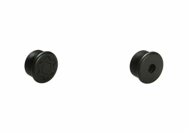
The .22LR End Cap is available in two variations: standard, with a smooth exterior and CMMG logo (.22LR End Cap LOGO), and QD (quick-detach), which has an attachment point machined into the exterior for attaching a QD sling. Installing the .22LR End Cap is made easy by securing the .22LR End Cap on the back of the lower receiver with a 3/8” hex wrench, in lieu of the buffer tube.
The .22LR End Cap with CMMG logo can be purchased separately for $24.95 and the QD End Cap for $29.95.
.22LR End Cap with CMMG logo (left) QD End Cap (Right)
BANSHEE lower groups and complete BANSHEE .22LR pistols are offered with the .22 LR End Cap preinstalled: the BANSHEE 100 Series comes with the .22 LR End Cap LOGO and the BANSHEE 200 and 300 Series come with the QD End Cap. MSRP on the complete BANSHEE pistols range from $799.95 to $1,024.95.
For more information on the .22LR End Cap and all BANSHEE models, please visit www.CMMGinc.com.
CMMG Guarantee:
All CMMG products are covered under the CMMG Lifetime Quality Guarantee. Conditioned on being a Limited Warranty of use, maintenance, and cleaning of the product in accordance with CMMG, Inc.’s instructions to be free of defects in material and workmanship. CMMG will repair, replace or substitute part(s) as determined in the sole and absolute discretion of CMMG Inc at no charge to the purchaser or provider. Complete limited warranty information can be found at CMMGinc.com/tech-support
About CMMG:
CMMG began in central Missouri in 2002 and quickly developed into a full-time business because of its group of knowledgeable and passionate firearms enthusiasts committed to quality and service. Its reputation was built on attention to detail, cutting edge innovation and the superior craftsmanship that comes from sourcing all their own parts. By offering high quality AR rifles, parts and accessories, CMMG’s commitment to top-quality products and professional service is as deep today as it was when it began.