An anonymous reader quotes a report from the Washington Post: A study published Monday in the Lancet found that the use of hearing aids can reduce the risk of cognitive decline by about half — 48 percent — for adults with more risk factors for dementia, such as elevated blood pressure, higher rates of diabetes, lower education and income, and those living alone. The study was presented at the Alzheimer’s Association International Conference in Amsterdam. […] Over a three-year period, the randomized controlled trial studied nearly 1,000 older adults, ages 70 to 84, in four sites in the United States. The participants included older adults in an ongoing study of cardiovascular health — Atherosclerosis Risk in Communities (ARIC) — and others who were healthier than the ARIC adults; both groups were from the same communities at each site.
When the two groups were combined, use of hearing aids was shown to have no significant effect on slowing cognitive changes. When the group at higher risk of dementia, the ARIC group, was analyzed separately, however, researchers found that hearing intervention — counseling with an audiologist and use of hearing aids — had a significant impact on reducing cognitive decline. Those considered at high risk for dementia were older and had lower cognitive scores, among other factors. When the groups were combined, the slower rate of cognitive decline experienced by the healthier participants may have limited any effect of hearing aids, the researchers suggested. Whether hearing treatment reduces the risk of developing dementia in the long term is still unknown. "That’s the next big question — and something we can’t answer yet," said Lin, who is also director of the Cochlear Center for Hearing and Public Health at Johns Hopkins University. He said he and his colleagues are planning a long-term follow-up study to attempt to answer that question.
There have many studies over the past decade to try to determine why people with hearing loss tend to have worse cognition, said Justin S. Golub, an associate professor of otolaryngology at Columbia University Irving Medical Center. One theory is that it requires a lot of effort for people with hearing loss to understand what others are saying — and that necessary brainpower leaves fewer cognitive resources to process the meaning of what was heard, he said. Another theory relates to brain structure. Research has shown that the temporal lobe of people with hearing loss tends to shrink quicker because it is not receiving as much auditory input from the inner ear. The temporal lobe is connected to other parts of the brain, and "that could have cascading influences on brain structure and function," said Golub, who was not part of the Lancet study. A third theory is that people with hearing loss tend to be less social and, as a result, have less cognitive stimulation, he said.
Eloquent has a lot of “hidden gems”. In this tutorial, let’s see how we can get the latest record from the hasMany Relationship in five different ways.
Let’s imagine we have transactions, and every transaction belongs to a category. The goal is to list the categories with the latest transaction for each of them.
While listing different methods, I will start from the worst one and go to the best method.
Method 1: Blade – Wrong Way (N+1 Query)
The first method is the most straightforward – to take care of the relationship in the Blade. But it’s the worst in terms of performance.
In the Controller, we just get the categories:
classHomeController
{
publicfunctionindex()
{
$categories=Category::take(10)->get();
returnview('categories',compact('categories'));
}
}
In the Blade, while viewing those categories, we load the latest transaction and take the first record.
<ul>
@foreach($categoriesas$category)
<li>
(last transaction: )
</li>
@endforeach
</ul>
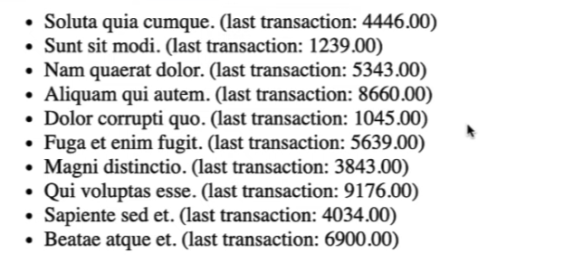
The result looks similar to the below image.
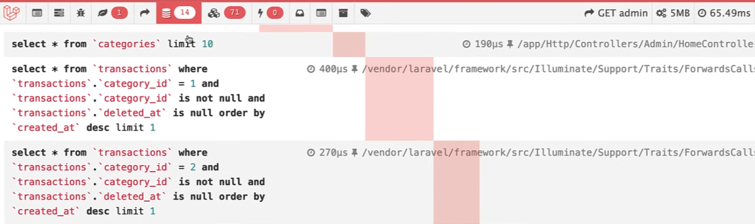
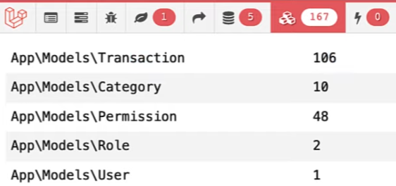
But with this method, we have an N+1 problem, which makes a database query for every category to get the transaction.
Method 2: Eager Loading with() – Still Wrong
In the second method, we fix the N+1 problem from the first method. Usually, it is done using the eager loading.
We load the transactions in the Controller using the with method.
And then, in the Blade, we don’t need to query the transactions. We can access the transactions from the collection and sort and get the first from that.
<ul>
@foreach($categoriesas$category)
<li>
(last transaction: )
</li>
@endforeach
</ul>
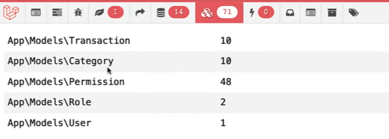
But this gives other problems. In the first method, we have ten transactions and categories loaded from the DB.
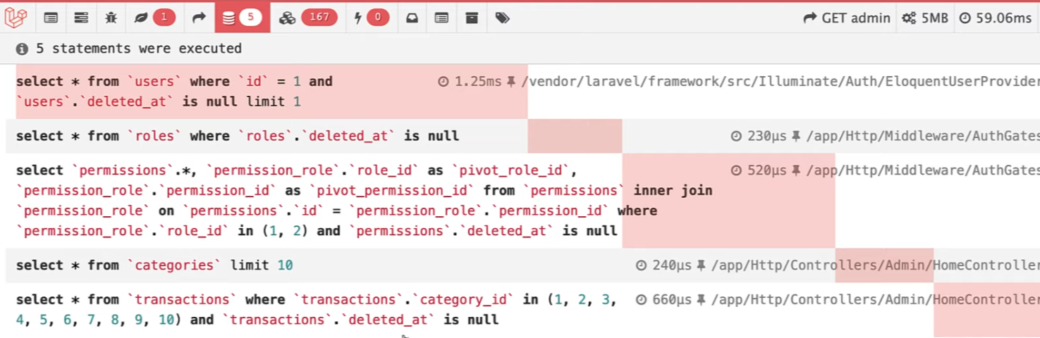
After a refresh, we have fewer queries which is great. Well, kinda.
But now we have loaded all the transactions for each category, which can get heavy on the RAM usage. This means we have improved performance in one place but decreased in another.
Method 3: Subquery
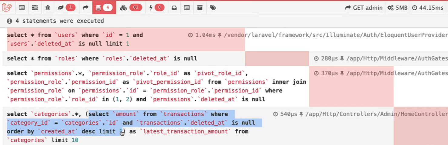
The third method is if you need precisely one field, so you don’t need all the transaction Model, for that, you might write a subquery.
In the query, we named the variable as latest_transaction_amount, so we just can use it in the Blade:
<ul>
@foreach($categoriesas$category)
<li>
(last transaction: )
</li>
@endforeach
</ul>
This way, we have only one query, but it can only be used when you need only one column from the relation table.
Method 4: Special Relation Method
But if you need the whole record, there is still a better way. Instead of using a transactions relation in the Category Model, we could create a special relation that would return the latest row.
And in the Blade, we don’t need to sort or do anything else.
<ul>
@foreach($categoriesas$category)
<li>
(last transaction: )
</li>
@endforeach
</ul>
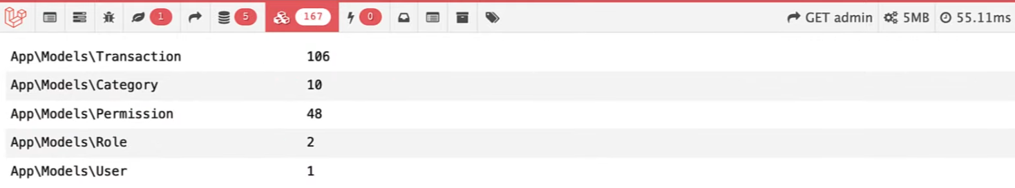
This makes only five queries which are good, but still loads all the transactions.
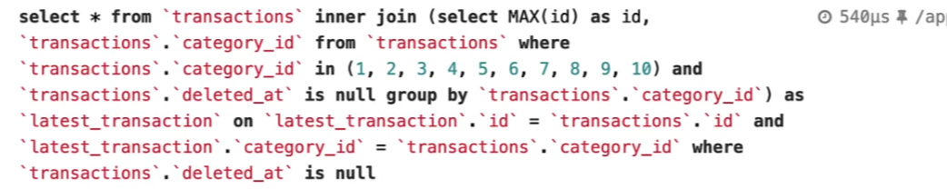
Method 5: New latestOfMany()
Since Laravel 8.42, there is a better way. It’s the same thing as latest_transaction in the fourth method, but instead of the latest, we need to use latestOfMany.
https://orasites-prodapp.cec.ocp.oraclecloud.com/content/published/api/v1.1/assets/CONT04A265851B14480BB7F962D7CB173DD0/native?cb=_cache_8b94&channelToken=32954b2a813146c9b9a4fa99364eba8eThis blog post introduces the new MySQL Configurator tool, available starting with MySQL Server 8.1.0.Planet MySQL
This is the stuff that kid dreams are made of. DreamTrack Builder headed to the top of an abandoned water slide and raced a bunch of Hot Wheels cars down its chute. A chase car sat at the back of the pack towing a GoPro camera. He also did a nighttime race and one with 50-cars.
Enlarge/ Take a peek inside the Ars vault with us!
Aurich Lawson | Getty Images
A bit over three years ago, just before COVID hit, we ran a long piece on the tools and tricks that make Ars function without a physical office. Ars has spent decades perfecting how to get things done as a distributed remote workforce, and as it turns out, we were even more fortunate than we realized because that distributed nature made working through the pandemic more or less a non-event for us. While other companies were scrambling to get work-from-home arranged for their employees, we kept on trucking without needing to do anything different.
However, there was a significant change that Ars went through right around the time that article was published. January 2020 marked our transition away from physical infrastructure and into a wholly cloud-based hosting environment. After years of great service from the folks at Server Central (now Deft), the time had come for a leap into the clouds—and leap we did.
There were a few big reasons to make the change, but the ones that mattered most were feature- and cost-related. Ars fiercely believes in running its own tech stack, mainly because we can iterate new features faster that way, and our community platform is unique among other Condé Nast brands. So when the rest of the company was either moving to or already on Amazon Web Services (AWS), we could hop on the bandwagon and take advantage of Condé’s enterprise pricing. That—combined with no longer having to maintain physical reserve infrastructure to absorb big traffic spikes and being able to rely on scaling—fundamentally changed the equation for us.
In addition to cost, we also jumped at the chance to rearchitect how the Ars Technica website and its components were structured and served. We were using a “virtual private cloud” setup at our previous hosting—it was a pile of dedicated physical servers running VMWare vSphere—but rolling everything into AWS gave us the opportunity to reassess the site and adopt some solid reference architecture.
Cloudy with a chance of infrastructure
And now, with that redesign having been functional and stable for a couple of years and a few billion page views (really!), we want to invite you all behind the curtain to peek at how we keep a major site like Ars online and functional. This article will be the first in a four-part series on how Ars Technica works—we’ll examine both the basic technology choices that power Ars and the software with which we hook everything together.
This first piece, which we’re embarking on now, will look at the setup from a high level and then focus on the actual technology components—we’ll show the building blocks and how those blocks are arranged. Another week, we’ll follow up with a more detailed look at the applications that run Ars and how those applications fit together within the infrastructure; after that, we’ll dig into the development environment and look at how Ars Tech Director Jason Marlin creates and deploys changes to the site.
Finally, in part 4, we’ll take a bit of a peek into the future. There are some changes that we’re thinking of making—the lure (and price!) of 64-bit ARM offerings is a powerful thing—and in part 4, we’ll look at that stuff and talk about our upcoming plans to migrate to it.
Ars Technica: What we’re doing
But before we look at what we want to do tomorrow, let’s look at what we’re doing today. Gird your loins, dear readers, and let’s dive in.
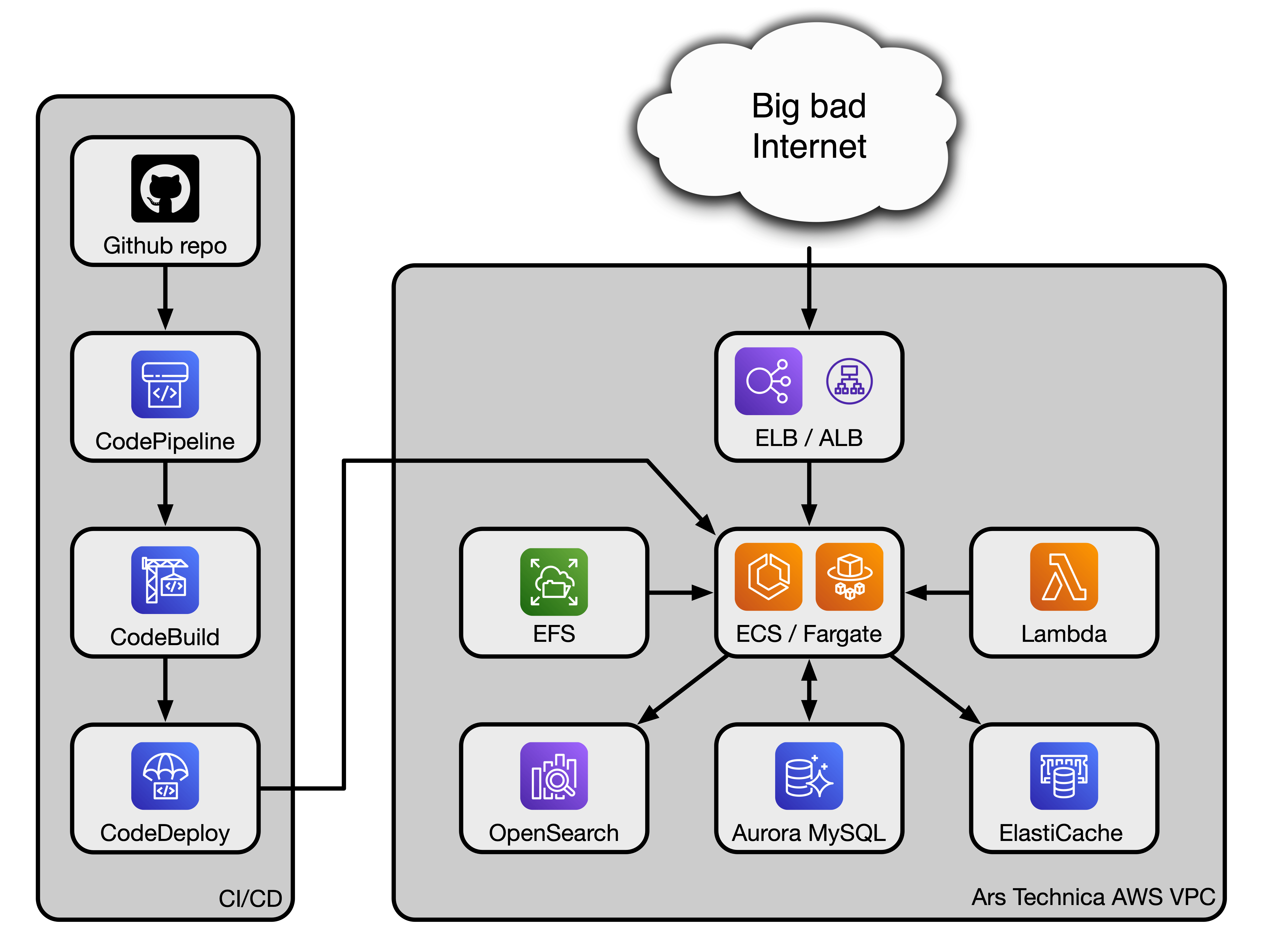
To start, here’s a block diagram of the specific AWS services Ars uses. It’s a relatively simple way to represent a complex interlinked structure:
Enlarge/ A high-level diagram of the Ars AWS setup.
Lee Hutchinson
Ars leans on multiple pieces of the AWS tech stack. We’re dependent on an Application Load Balancer (ALB) to first route incoming visitor traffic to the appropriate Ars back-end service (more on those services in part 2). Downstream of the ALB, we use two services called Elastic Container Services (ECS) and Fargate in conjunction with each other to spin up Docker-like containers to do work. Another service, Lambda, is used to run cron jobs for the WordPress application that forms the core of the Ars website (yes, Ars runs WordPress—we’ll get into that in part 2).
Here’s an example of a product invention that does a lot with a little. The Jeri-Rigg is a polyester webbing strap that terminates in a hook or an eye, your choice. The strap can be looped around anything and the hook or eye drawn through the slit in the strap, creating a tie-down point.
The idea, writes Michigan-based inventor Jerry Hill, is to avoid doing what’s shown in the two photos below when there’s no suitable tie-down point:
That’s not a secure connection, as you might find out the hard way. Thus Hill’s solution:
The applications are numerous:
"The Jeri-Rigg (Eye version) has a tested workload between 1100-3000 pounds and has a breaking strength between 3300-9000 pounds and comes in 4 sizes; the "Hook" version has a working load between 280-500 pounds and a breaking strength between 840-1500 pounds and comes in three sizes."
"The strap is made of 100% high strength polyester and the eyes are made of 316 marine grade stainless steel. The hooks are made of 1020 steel, then powder coated to protect them from corrosion."
"It is designed to handle the toughest of elements and conditions."
Prices start at $17 for the eye version and $19 for the hook version.
When working with data in Python, one of the most powerful tools at your disposal is the pandas DataFrame.
A DataFrame is a two-dimensional data structure, which essentially looks like a table with rows and columns. This versatile data structure is widely used in data science, machine learning, and scientific computing, among other data-intensive fields. It combines the best features of SQL tables and spreadsheets, offering a more efficient way to work with large volumes of structured data.
As you dive deeper into pandas, you’ll find that DataFrames give you flexibility and high performance, allowing you to easily perform various operations, such as filtering, sorting, and aggregating data.
DataFrames also support a wide range of data types, from numerical values to timestamps and strings, making it suitable for handling diverse data sources.
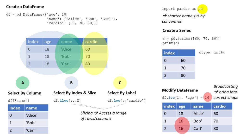
You can easily create a DataFrame object using the pd.DataFrame() function, providing it with data in several formats, such as dictionaries, NumPy arrays, or even CSV files.
In this article, you can familiarize yourself with their key components and features. Understanding how to index, slice, and concatenate DataFrames will enable you to manipulate data efficiently and optimize your workflow.
Moreover, pandas offers a wealth of built-in functions and methods, empowering you to perform complex data analysis and visualization tasks.
Pandas DataFrame Object Fundamentals
Pandas is a popular Python library for handling and analyzing data. One of the core components in Pandas is the DataFrame object.
A DataFrame can be thought of as a two-dimensional table with columns and rows, which enables the storage and manipulation of data.
Creating a DataFrame is simple, you can start by importing the Pandas library:
This creates a DataFrame with columns A, B, and C, and rows containing the values from the Numpy array.
From CSV File
Lastly, you can create a DataFrame from a CSV file. To do this, you can use the pd.read_csv() function, which reads the CSV file and returns a DataFrame:
csv_df = pd.read_csv("your_file.csv")
Replace "your_file.csv" with the location and name of your CSV file. This will create a DataFrame containing the data from the CSV file.
Accessing and Manipulating Data
Selecting Rows and Columns
To select specific rows and columns from a DataFrame, you can use the iloc and loc methods. The iloc method is used for integer-based indexing, while loc is used for label-based indexing.
For example, to select the first row of data using iloc, you can do:
import pandas as pd

# Create a DataFrame
data = {'A': [1, 2], 'B': [3, 4]}
df = pd.DataFrame(data)

# Select the first row using iloc
first_row = df.iloc[0]
To select a specific column, you can use the column name as follows:
# Select column 'A' using column name
column_a = df['A']
You can also use the loc method to select rows and columns based on labels:
# Select first row of data using loc with index label
first_row_label = df.loc[0]
Slicing
When you need to select a range of rows or columns, slicing comes in handy. Slicing works similarly to Python lists, where you indicate the start and end index separated by a colon. Remember that the end index is exclusive.
For instance, if you want to select the first two rows of a DataFrame, you can slice like this:
# Slice the first two rows
first_two_rows = df.iloc[0:2]

# Slice the first column using iloc
first_column = df.iloc[:, 0:1]
Filtering the DataFrame can be done using conditions and the query or eval method. To filter rows based on specific column values, you can use the query method:
# Filter rows where column 'A' is greater than 1
filtered_rows = df.query("A > 1")
Alternatively, you can use the eval() method with conditional statements:
# Filter rows where column 'A' is greater than 1 using eval method
condition = df.eval('A > 1')
filtered_rows_eval = df[condition]
Modifying Data
You can modify the data in your DataFrame by assigning new values to specific cells, rows, or columns. Directly assigning a value to a cell, using the index and column name:
# Update the value of the cell at index 0 and column 'A'
df.loc[0, 'A'] = 5
To modify an entire column or row, simply reassign the new values to the column or row using the column name or index:
# Update the values of column 'A'
df['A'] = [6, 7]

# Update the values of the first row
df.loc[0] = [8, 9]
In summary, you can efficiently access and manipulate the data in your DataFrame using various methods such as iloc, loc, query, eval, and slicing with indexing.
Indexing and Alignment
Index Objects
In a pandas DataFrame, index objects serve to identify and align your data. Index objects can be created using the Index constructor and can be assigned to DataFrame columns. They consist of an immutable sequence used for indexing and alignment, making them an essential part of working with pandas.
To create an index object from a Python dict or a list of years, you can use the following code:
To set the index of your DataFrame, use the set_index() method, which allows you to set one or multiple columns as the index. If you want to revert the index back to a default integer-based index, use the reset_index() method:
import pandas as pd

df = pd.DataFrame({'Year': [2010, 2011, 2012],
                   'Value': [100, 200, 300]})

# Set the Year column as the index
df.set_index('Year', inplace=True)

# Reset the index
df.reset_index(inplace=True)
Hierarchical Indexing
Hierarchical indexing (also known as multi-level indexing) allows you to create a DataFrame with multiple levels of indexing. You can construct a MultiIndex using the pd.MultiIndex.from_tuples() method.
This can help you work with more complex data structures:
import pandas as pd

index_tuples = [('A', 'X'), ('A', 'Y'), ('B', 'X'), ('B', 'Y')]
multi_index = pd.MultiIndex.from_tuples(index_tuples)

# Create a new DataFrame with the MultiIndex
columns = ['Value']
data = [[1, 2, 3, 4]]
df = pd.DataFrame(data, columns=multi_index)
Alignment and Reindexing
When performing operations on data within a DataFrame, pandas will automatically align the data using the index labels. This means that the order of the data is not important, as pandas will align them based on the index.
To manually align your DataFrame to a new index, you can use the reindex() method:
import pandas as pd

original_index = pd.Index(['A', 'B', 'C'])
new_index = pd.Index(['B', 'C', 'D'])

# Create a DataFrame with the original index
df = pd.DataFrame({'Value': [1, 2, 3]}, index=original_index)

# Align the DataFrame to the new index
aligned_df = df.reindex(new_index)
Operations on Dataframes
Arithmetic Operations
In pandas, you can easily perform arithmetic operations on DataFrames, such as addition, subtraction, multiplication, and division. Use the pandas methods like add() and div() to perform these operations.
You can compare elements in DataFrames using methods like eq() for equality and compare() for a more comprehensive comparison. This is useful for tasks like data manipulation and indexing. For instance:
Pandas provides several aggregation methods like sum() and corr() to help you summarize and analyze the data in your DataFrame. These methods are especially helpful when dealing with NaN values.
For example:
import pandas as pd
import numpy as np

# Create a DataFrame with NaN values
df = pd.DataFrame({'A': [1, 2, np.nan], 'B': [3, 4, np.nan]})

# Calculate the sum and correlation of each column
result_sum = df.sum()
result_corr = df.corr()
String Operations
Pandas also supports a wide range of string operations on DataFrame columns, such as uppercasing and counting the occurrences of a substring. To apply string operations, use the .str accessor followed by the desired operation.
Here’s an example using the upper() and count(sub) string methods:
import pandas as pd

# Create a DataFrame with string values
df = pd.DataFrame({'A': ['apple', 'banana'], 'B': ['cherry', 'date']})

# Convert all strings to uppercase and count the occurrences of 'a'
result_upper = df['A'].str.upper()
result_count = df['A'].str.count('a')
Handling Missing Data
When working with Pandas DataFrames, it’s common to encounter missing data. This section will cover different techniques to handle missing data in your DataFrames, including detecting null values, dropping null values, and filling or interpolating null values.
Detecting Null Values
To identify missing data in your DataFrame, you can use the isnull() and notnull() functions. These functions return boolean masks indicating the presence of null values in your data.
To check if any value is missing, you can use the any() function, while all() can be used to verify if all values are missing in a specific column or row.
import pandas as pd

# Create a DataFrame with missing values
data = {'A': [1, 2, None], 'B': [4, None, 6]}
df = pd.DataFrame(data)

null_mask = df.isnull()
print(null_mask)

# Check if any value is missing in each column
print(null_mask.any())

# Check if all values are missing in each row
print(null_mask.all(axis=1))
Dropping Null Values
If you need to remove rows or columns with missing data, the dropna() function can help. By default, dropna() removes any row with at least one null value. You can change the axis parameter to drop columns instead. Additionally, you can use the how parameter to change the criteria for dropping data.
For example, how='all' will only remove rows or columns where all values are missing.
# Drop rows with missing values
df_clean_rows = df.dropna()

# Drop columns with missing values
df_clean_columns = df.dropna(axis=1)

# Drop rows where all values are missing
df_clean_all = df.dropna(how='all')
Filling and Interpolating Null Values
Instead of dropping null values, you can fill them with meaningful data using the fillna() function. The fillna() function allows you to replace missing data with a specific value, a method such as forward fill or backward fill, or even fill with the mean or median of the column.
# Fill missing values with zeros
df_fill_zeros = df.fillna(0)

# Forward fill missing values
df_fill_forward = df.fillna(method='ffill')

# Fill missing values with column mean
df_fill_mean = df.fillna(df.mean())
For a more advanced approach, you can use the interpolate() function to estimate missing values using interpolation methods, such as linear or polynomial.
In this example, the Dataframes df1 and df2 have been stacked vertically, and the ignore_index parameter has been used to reindex the resulting dataframe.
Merging
Merging allows you to combine data based on common columns between your Dataframes. The merge function allows for various types of merges, such as inner, outer, left, and right.
left = pd.DataFrame({'key': ['K0', 'K1'], 'A': ['A0', 'A1'], 'B': ['B0', 'B1']})
right = pd.DataFrame({'key': ['K0', 'K1'], 'C': ['C0', 'C1'], 'D': ['D0', 'D1']})

result = pd.merge(left, right, on='key')
In this example, the Dataframes left and right are merged based on the common column “key.”
Joining
Joining is another method to combine Dataframes based on index. The join method allows for similar merging options as the merge function.
left = pd.DataFrame({'A': ['A0', 'A1'], 'B': ['B0', 'B1']}, index=['K0', 'K1'])
right = pd.DataFrame({'C': ['C0', 'C1'], 'D': ['D0', 'D1']}, index=['K0', 'K2'])

result = left.join(right, how='outer')
In this example, the Dataframes left and right are joined based on index, and the how parameter is set to ‘outer’ for an outer join.
Reshaping DataFrames is a common task when working with pandas. There are several operations available to help you manipulate the structure of your data, making it more suitable for analysis. In this section, we will discuss pivoting, melting, stacking, and unstacking.
Pivoting
Pivoting is a technique that allows you to transform a DataFrame by reshaping it based on the values of specific columns. In this process, you can specify an index, columns, and values to create a new DataFrame. To perform a pivot, you can use the pivot() function.
Here, population is used as the index, instance determines the columns, and the values in the point column will be the new DataFrame’s data. This transformation is helpful when you want to restructure your data for improved readability or further analysis.
Melting
Melting is the opposite of pivoting, where you “melt” or “gather” columns into rows. The melt() function helps you achieve this. With melting, you can specify a list of columns that would serve as id_vars (identifier variables) and value_vars (value variables).
The melt() function combines the instance and point columns into a single column, while keeping the population column as the identifier.
Stacking
Stacking is another operation that allows you to convert a DataFrame from a wide to a long format by stacking columns into a multi-level index. You can use the stack() method to perform stacking.
For instance:
stacked_df = df.stack()
This will create a new DataFrame with a multi-level index where the additional level is formed by stacking the columns of the original DataFrame. This is useful when you want to analyze your data in a more hierarchical manner.
Unstacking
Unstacking is the inverse operation of stacking. It helps you convert a long-format DataFrame with a multi-level index back into a wide format. The unstack() method allows you to do this. For example:
unstacked_df = stacked_df.unstack()
This will create a new DataFrame where the multi-level index is converted back into columns. Unstacking is useful when you want to revert to the original structure of the data or prepare it for visualization.
Advanced Features
In this section, we’ll explore some advanced features available in Pandas DataFrame, such as Time Series Analysis, Groupby and Aggregate, and Custom Functions with Apply.
Time Series Analysis
Time Series Analysis is a crucial component for handling data with a time component. With Pandas, you can easily work with time-stamped data using pd.to_datetime(). First, ensure that the index of your DataFrame is set to the date column.
Now that your DataFrame has a DateTimeIndex, you can access various Datetime properties like year, month, day, etc., by using df.index.[property]. Some operations you can perform include:
Resampling: You can resample your data using the resample() method. For instance, to resample the data to a monthly frequency, execute df.resample('M').mean().
Rolling Window: Calculate rolling statistics like rolling mean or rolling standard deviation using the rolling() method. For example, to compute a 7-day rolling mean, utilize df.rolling(7).mean().
You can watch our Finxter explainer video here:
Groupby and Aggregate
The groupby() method helps you achieve powerful data aggregations and transformations. It involves splitting data into groups based on certain criteria, applying a function to each group, and combining the results.
Here’s how to use this method:
Split: Group your data using the groupby() function by specifying the column(s) to group by. For example, grouped_df = df.groupby('type').
Apply: Apply an aggregation function on the grouped data, like mean(), count(), sum(), etc. For instance, grouped_df_mean = grouped_df.mean().
Combine: The result is a new DataFrame with the groupby column as the index and the aggregated data.
You can also use the agg() function to apply multiple aggregate functions at once, or even apply custom functions.
You can apply custom functions to DataFrame columns or rows with apply(). This method allows you to apply any function that you define or that comes from an external library like NumPy.
For instance, to apply a custom function to a specific column:
def custom_function(value):
    # Your custom logic here
    return processed_value

df['new_column'] = df['column'].apply(custom_function)
It’s also possible to apply functions element-wise with applymap(). This method enables you to process every element in your DataFrame while keeping its structure:
def custom_function_elementwise(value):
    # Your custom logic here
    return processed_value

df = df.applymap(custom_function_elementwise)
By leveraging these advanced features, you can effectively work with complex data using Pandas DataFrames, while handling operations on Time Series data, group-based aggregations, and custom functions.
Remember to consider features such as dtype, data types, loc, ge, name, diff, count, strings, and r while working with your data, as these can significantly impact your analysis’ efficiency and accuracy.
Optimization and Performance
In this section, we’ll discuss some effective strategies that can help you improve the efficiency of your code.
Data Types Conversion
Use the appropriate data types for your DataFrame columns. Converting objects to more specific data types can reduce memory usage and improve processing speed.
Use the astype() method to change the data type of a specific column:
You might also want to consider converting pandas Series to numpy arrays using the to_numpy() function for intensive numerical computations. This can make certain operations faster:
numpy_array = df['column_name'].to_numpy()
Memory Optimization
Another way to enhance performance is by optimizing memory usage. Check the memory consumption of your DataFrame using the info() method:
df.info(memory_usage='deep')
For large datasets, consider using the read_csv() function’s low_memory,dtype, usecols, and nrows options to minimize memory consumption while importing data:
Leveraging parallel processing can significantly decrease the time required for computations on large DataFrames. Make use of pandas’ apply() function in combination with multiprocessing for parallel execution of functions across multiple cores:
import pandas as pd
from multiprocessing import cpu_count, Pool

def parallel_apply(df, func):
    n_cores = cpu_count()
    data_split = np.array_split(df, n_cores)
    pool = Pool(n_cores)
    result = pd.concat(pool.map(func, data_split))
    pool.close()
    pool.join()
    return result

df['new_column'] = parallel_apply(df['column_name'], some_function)
Dask
Dask is a parallel computing library for Python that can significantly speed up pandas’ operations on large DataFrames. Dask’s DataFrame object is similar to pandas’ DataFrame, but it partitions the data across multiple cores or even clusters for parallel processing. To use Dask, simply replace your pandas import with Dask:
import dask.dataframe as dd
Then, you can read and process large datasets as you would with pandas:
ddf = dd.read_csv('large_file.csv')
By implementing these optimization techniques, you’ll be able to efficiently work with large DataFrames, ensuring optimal performance and minimizing processing time.
Frequently Asked Questions
How to create a DataFrame from a list?
To create a DataFrame from a list, you can use the pandas.DataFrame() function. First, import the pandas library:
import pandas as pd
Then, create a list of data:
data = [['A', 10], ['B', 20], ['C', 30]]
Finally, create the DataFrame using the pd.DataFrame() function:
DataFrames are versatile data structures that allow for easy manipulation and analysis of data. Some common operations include selecting a specific column or row, filtering data, or applying functions to the data.
To add a row to a DataFrame, you can use the loc[] indexer:
df.loc[len(df.index)] = ['E', 50]
print(df)
This will add a new row with the values ‘E’ and 50 to the DataFrame.
How to save a DataFrame as CSV file?
To save a DataFrame as a CSV file, use the to_csv() method:
df.to_csv('data.csv', index=False)
This will save the DataFrame to a CSV file named ‘data.csv’ in your current working directory. The index=False parameter tells pandas not to include the index column in the CSV file.
Most USB-C docks are pretty nondescript. But RayCue’s retro docks borrow their looks from the OG Apple Macintosh. The 128K Dock looks like a 1980s Mac, and packs USB-A, USB-C, HDMI, Ethernet, and headphone jacks. It’s also a Bluetooth speaker, a memory card reader, and a digital photo frame. The simpler Pocket dock looks like a tiny Mac keyboard.
Introducing LaravelGPT, a tool designed to simplify the integration of OpenAI’s ChatGPT with your Laravel applications. This package offers a seamless connection to the OpenAI Chat Completions API, even supporting Function Calling. Forget the complications of crafting the correct JSON schema – LaravelGPT does the work for you. Say goodbye to dense, hard-to-read code, and start building the applications of the future! With LaravelGPT, you can truly unleash the power of ChatGPT in your applications, setting the stage for innovation and advanced user interaction.
Installation
You can install the package via composer:
composer require maltekuhr/laravel-gpt
Next you need to configure your OpenAI API Key and Organization ID. You can find both in the OpenAI Dashboard.
You guys, it’s only a matter of time before the rioters return to our big cities for another round of destruction. Usually, for some reason, it happens during an election year, so look for them to arrive in a few month’s time, maybe a year tops.


 A DataFrame is a two-dimensional data structure, which essentially looks like a table with rows and columns. This versatile data structure is widely used in data science, machine learning, and scientific computing, among other data-intensive fields. It combines the best features of SQL tables and spreadsheets, offering a more efficient way to work with large volumes of structured data.


