Month: October 2024

https://media.notthebee.com/articles/6723bb0ebb9af6723bb0ebb9b0.jpg

Happy Halloween, y’all. JD Vance just did 3+ hours with Rogan and we’ve got the whole thing for you here.

Not the Bee

https://blog.jetbrains.com/wp-content/uploads/2024/10/compact.png

Maybe you’ve heard complicated-sounding phrases such as ‘“Students t-test”, “regression models”, “support vector machines”, and so on. You might think there’s so much you need to learn before you can explore and understand your data, but I am going to show you two tools to help you go faster. These are summary statistics and graphs.

Summary statistics and graphs/plots are used by new and experienced data scientists alike, making them the perfect building blocks for exploring data.

We will be working with this dataset available from Kaggle if you’d like to follow along. I chose this dataset because it has several interesting properties, such as multiple continuous and categorical variables, missing data, and a variety of distributions and skews. I’ll explain each variable I work with and why I chose each one to show you the tools you can apply to your chosen data set.

In our previous blog posts, we looked at where to get data from and bring that data into PyCharm. You can look at steps 1 and 2 from our blog post entitled 7 ways to use Jupyter notebooks in PyCharm to create a new Jupyter notebook and import your data as a CSV file if you need a reminder. You can use the dataset I linked above or pick your own for this walkthrough.

We’re going to be using the pandas library in this blog post, so to ensure we’re all on the same page, your code should look something like the following block in a Jupyter notebook –  you’ll need to change the spreadsheet name and location to yours, though. Make sure you’ve imported matplotlib, too, as we will be using that library to explore our data.

import pandas as pd
import matplotlib as plt


df = pd.read_csv('../data/AmesHousing.csv')
df

When you run that cell, PyCharm will show you your DataFrame, and we can get started.

Try PyCharm Professional for free

Summary statistics

When we looked at where to get data from, we discussed continuous and categorical variables. We can use Jupyter notebooks inside PyCharm to generate different summary statistics for these, and, as you might have already guessed, the summary statistics differ depending on whether the variables are continuous or categorical.

Continuous variables summary statistics

First, let’s see how we can view our summary statistics. Click on the small bar graph icon on the right-hand side of your DataFrame and select Compact:

Let me give you a little tip here if you’re unsure which variables are continuous and which are categorical, PyCharm shows different summary statistics for each one. The ones with the mini graphs (blue in this screenshot) are continuous, and those without are categorical.

This data set has several continuous variables, such as Order, PID, MS SubClass, and more, but we will focus on Lot Frontage first. That is the amount of space at the front of the property.

The summary statistics already give us some clues:

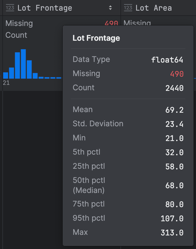
There’s a lot of data here, so let’s break it down and explore it to understand it better. Immediately, we can see that we have missing data for this variable; that’s something we want to note, as it might mean we have some issues with the dataset, although we won’t go into that in this blog post!

First, you can see the little histogram in blue in my screenshot, which tells us that we have a positive skew in our data because the data tails off to the right. We can further confirm this with the data because the mean is slightly larger than the median. That’s not entirely surprising, given we’d expect the majority of lot frontages to be of a similar size, but perhaps there are a small number of luxury properties with much bigger lot frontages that are skewing our data. Given this skew, we would be well advised not to use the standard deviation as a measure of dispersion because that is calculated by using all data points, so it’s affected by outliers, which we know we have on one side of our distribution.

Next, we can calculate our interquartile range as the difference between our 25th percentile of 58.0 and our 75th percentile of 80.0, giving us an interquartile range of 22.0. Alongside the interquartile range, it’s helpful to consider the median, the middle value in our data, and unlike the mean, it is not based on every data point. The median is more appropriate for Lot Frontage than the mean because it’s not affected by the outliers we know we have.

Since we’re talking about the median and interquartile range, it is worth saying that box plots are a great way to represent these values visually. We can ask JetBrains AI Assistant to create one for us with a prompt such as this:

Create code using matplotlib for a box plot for  ‘Lot Frontage’. Assume we have all necessary imports and the data exists.

Here’s the code that was generated:

plt.figure(figsize=(10, 6))
plt.boxplot(df['Lot Frontage'].dropna(), vert=False)
plt.title('Box Plot of Lot Frontage')
plt.xlabel('Lot Frontage')
plt.show()

When I click Accept and run, we get our box plot:

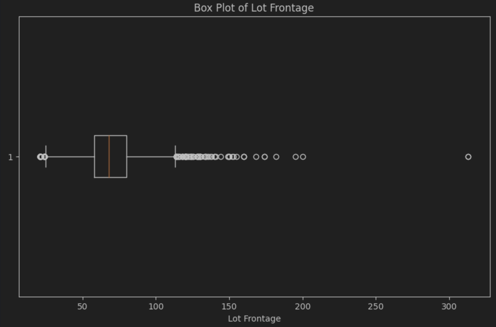
The median is the line inside the box, which, as you can see, is slightly to the left, confirming the presence of the positive or right-hand skew. The box plot also makes it very easy to see a noticeable number of outliers to the right of the box, known as “the tail”. That’s the small number of likely luxury properties that we suspect we have.

It’s important to note that coupling the mean and standard deviation or the median and IQR gives you two pieces of information for that data: a central tendency and the variance. For determining the central tendency, the mean is more prone to being affected by outliers, so it is best when there is no skew in your data, whereas the median is more robust in that regard. Likewise, for the variation, the standard deviation can be affected by outliers in your data. In contrast, the interquartile range will always tell you the distribution of the middle 50% of your data. Your goals determine which measurements you want to use. 

Categorical variables summary statistics

When it comes to categorical variables in your data, you can use the summary statistics in PyCharm to find patterns. At this point, we need to be clear that we’re talking about descriptive rather than inferential statistics. That means we can see patterns, but we don’t know if they are significant.

Some examples of categorical data in this data set include MS Zoning, Lot Shape, and House Style. You can gain lots of insights just by looking through your data set. For example, looking at the categorical variable Neighborhood, the majority are stated as Other in the summary statistics with 75.8%. This tells you that there might well be a lot of categories in Neighborhood, which is something to bear in mind when we move on to graphs. 

As another example, the categorical variable House Style states that about 50% of the houses are one-story, while 30% are two-story, leaving 20% that fall into some other category that you might want to explore in more detail. You can ask JetBrains AI for help here with a prompt like:

Write pandas code that tells me all the categories for ‘House Style’ in my DataFrame ‘df’, which already exists. Assume we have all the necessary imports and that the data exists.

Here’s the resulting code:

unique_house_styles = df['House Style'].unique()


print("Unique categories for 'House Style':")
print(unique_house_styles)

When we run that we can see that the remaining 20% is split between various codes that we might want to research more to understand what they mean:

Unique categories for ‘House Style’:

['1Story' '2Story' '1.5Fin' 'SFoyer' 'SLvl' '2.5Unf' '1.5Unf' '2.5Fin']

Have a look through the data set at your categorical variables and see what insights you can gain!

Before we move on to graphs, I want to touch on one more piece of functionality inside PyCharm that you can use to access your summary statistics called Explain DataFrame. You can access it by clicking on the purple AI icon on the top-right of the DataFrame and then choosing AI Actions | Explain DataFrame.

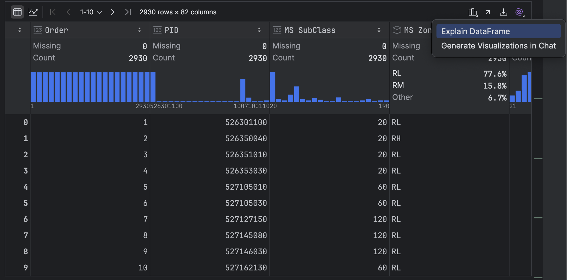
JetBrains AI lists out your summary statistics but may also add some code snippets that are helpful for you to get your data journey started, such as how to drop missing values, filter rows based on a condition, select specific columns, as well as group and aggregate data. 

Graphs

Graphs or plots are a way of quickly getting patterns to pop out at you that might not be obvious when you’re looking at the numbers in the summary statistics. We’re going to look at some of the plots you can get PyCharm to generate to help you explore your data.

First, let’s revisit our continuous variable, Lot Frontage. We already learned that we have a positive or right-hand skew from the mini histogram in the summary statistics, but we want to know more! 

In your DataFrame in PyCharm, click the Chart View icon on the left-hand side:

Now click the cog on the right-hand side of the chart that says Show series settings and select the Histogram plot icon on the far right-hand side. Click x to clear the values in the X axis and Y axis and then select Lot Frontage with group and sort for the X axis and Lot Frontage with count for the Y axis:

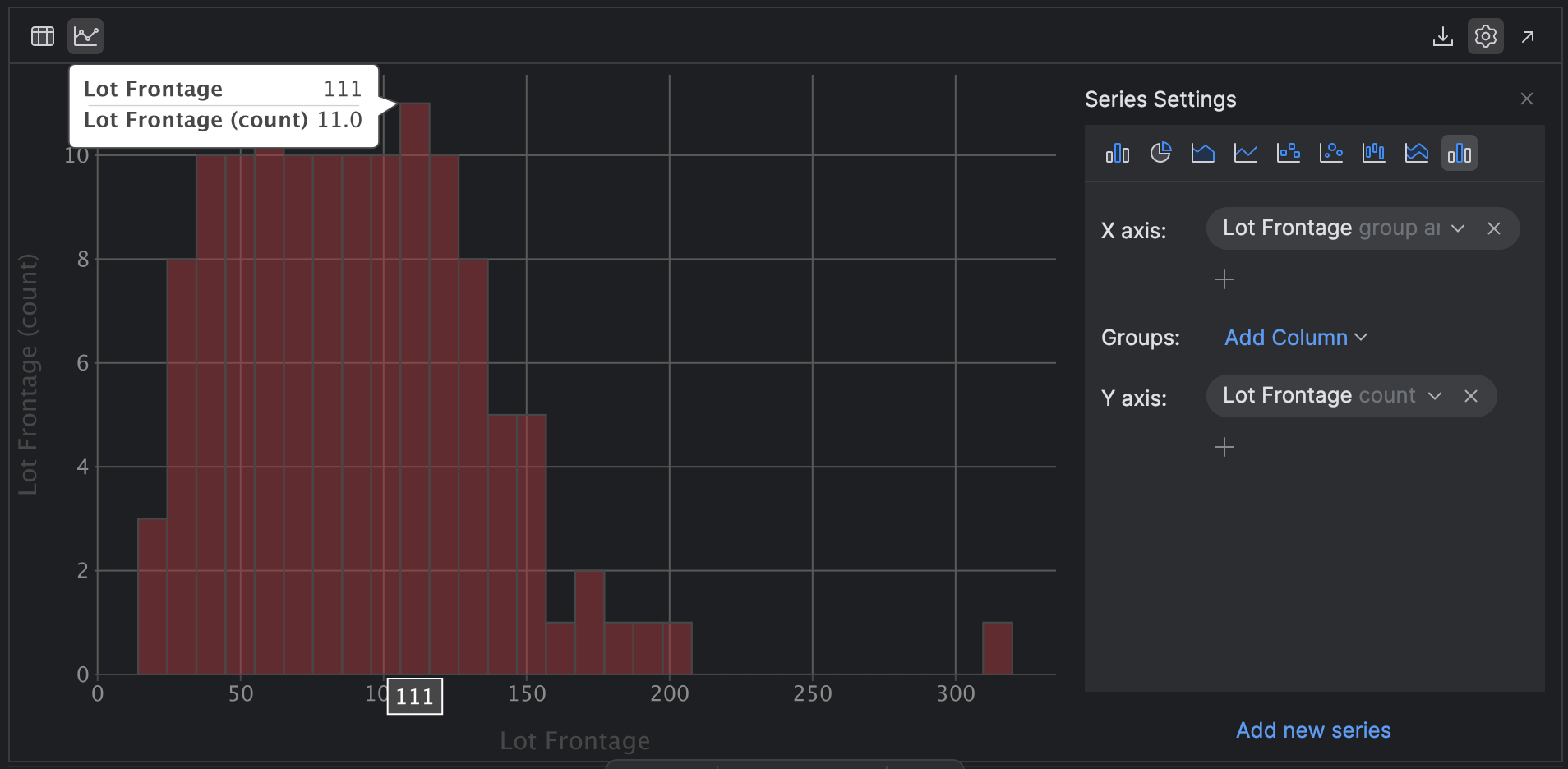
PyCharm generates the same histogram as you see in the summary settings, but we didn’t have to write a single line of code. We can also explore the histogram and mouse over data points to learn more. 

Let’s take it to the next level while we’re here. Perhaps we want to see if the condition of the property, as captured by the Overall Cond variable, predicts the sale price.

Change your X axis SalePrice group and sort and your Y axis to SalePrice count and then add the group Overall Cond:

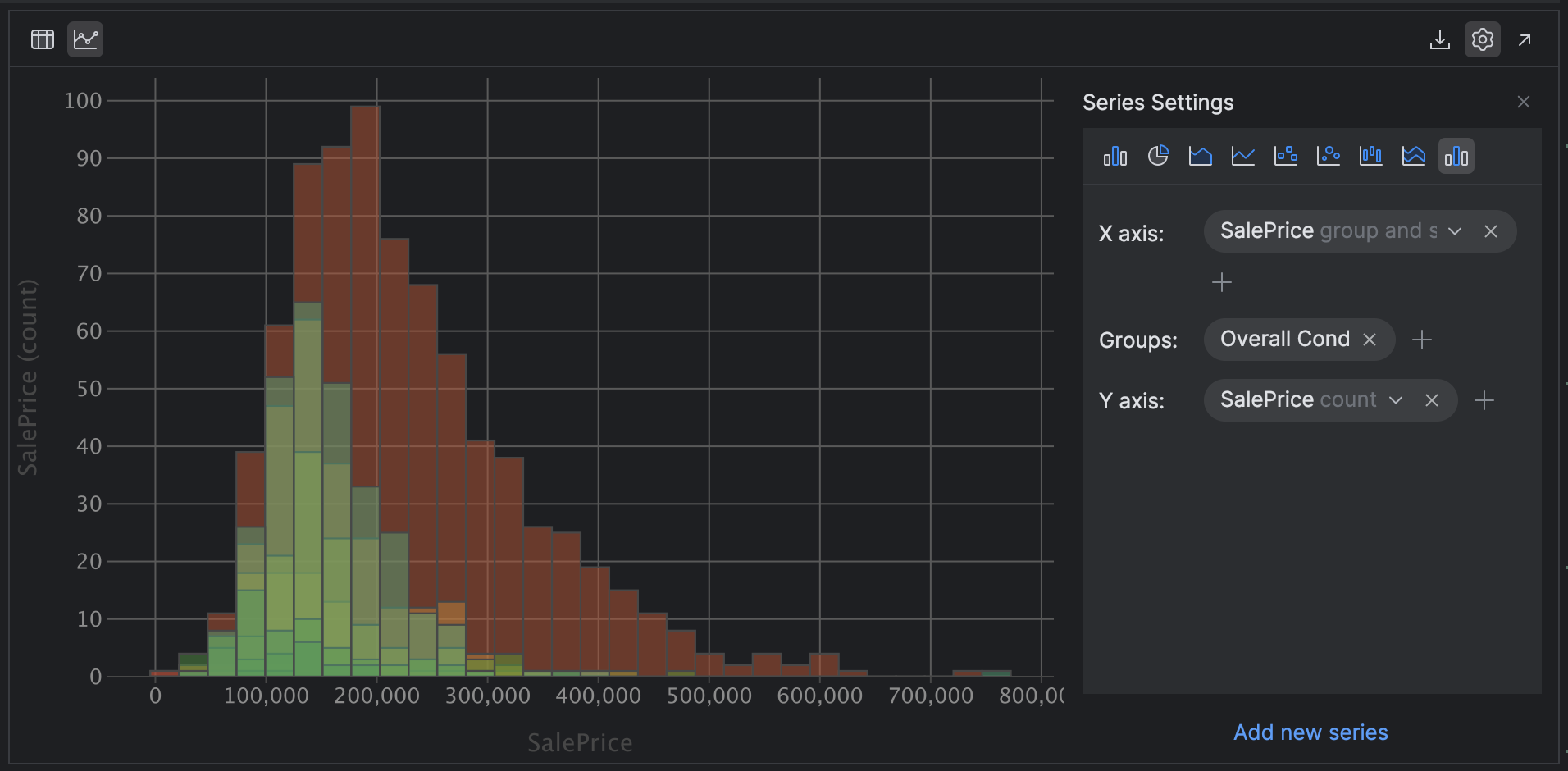
Looking at this chart, we can hypothesize that the overall condition of the property is indeed a predictor of the sale price, as the distribution and skew are remarkably similar. One small note is that grouping histograms like this works best when you have a smaller number of categories. If you change Groups to Neighborhood, which we know has many more categories, it becomes much harder to view! 

Moving on, let’s stick with PyCharm’s plotting capabilities and explore bar graphs. These are a companion to frequency charts such as histograms, but can also be used for categorical data. Perhaps you are interested in Neighbourhood (a categorical variable) in relation to SalesPrice.

Click the Bar [chart] icon on the left-hand side of your series setting, then select Neighbourhood as Categories and SalesPrice with the median as the Values:

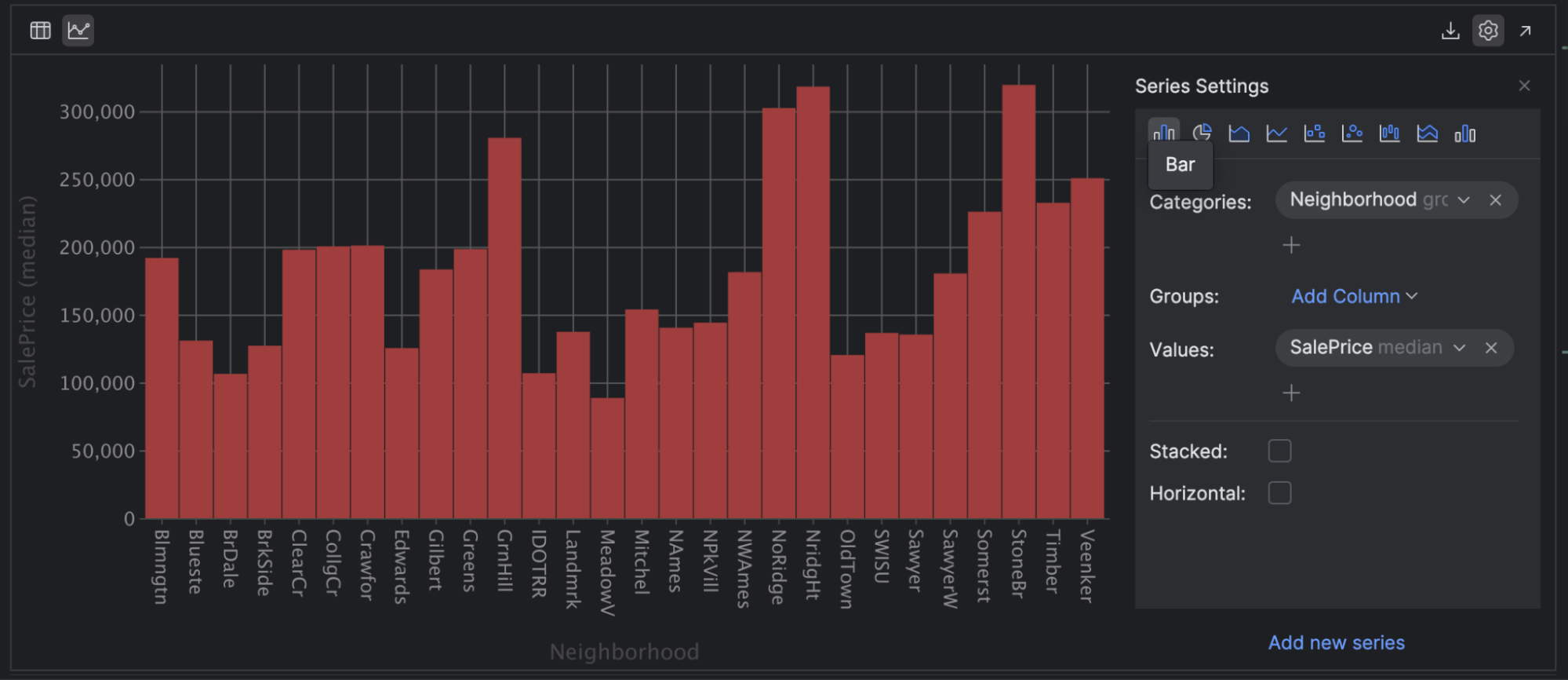
This helps us understand the neighborhoods with the most expensive and cheapest housing. I chose the median for the SalesPrice as it’s less susceptible to outliers in the data. For example, I can see that housing in Mitchel is likely to be substantially cheaper than in NoRidge. 

Line plots are another useful plot for your toolkit. You can use these to demonstrate trends between continuous variables over a period of time. For example, select the Line [graph] icon and then choose Year Built as the X axis and SalePrice with the mean as the Y axis:

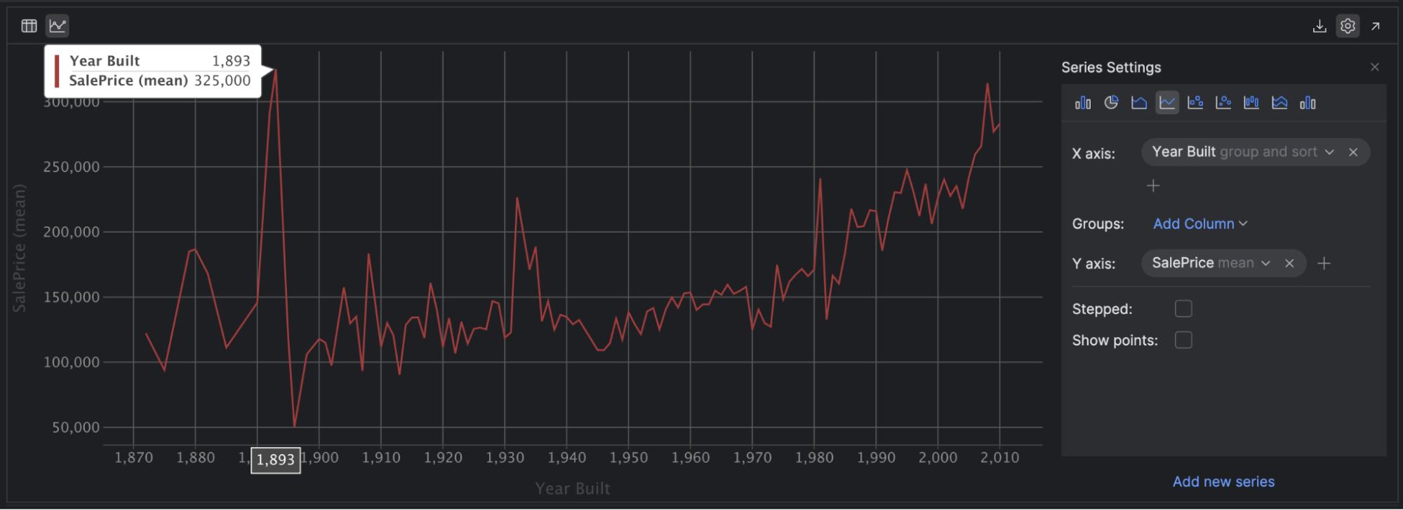
This suggests a small positive correlation between the year the house was built and the price of the house, especially after 1950. If you’re feeling adventurous, remove the mean from SalePrice and see how your graph changes when it has to plot every single price! 

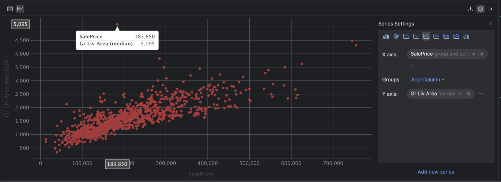
The last plot I’d like to draw your attention to is scatter plots. These are a great way to see a relationship between two continuous variables and any correlation between them. A correlation shows the strength of a relationship between two variables. To dig deeper, check out this beginner-friendly overview from Real Python.

For example, if we set our X axis to SalePrice and our Y axis to Gr LivArea, we can see that there is a positive correlation between the two variables, and we can also easily spot some outliers in our data, including a couple of houses with a lower sale price but a huge living area!

Summary

Here’s a reminder of what we’ve covered today. You can access your summary statistics in PyCharm either through Explain DataFrame with JetBrains AI or by clicking on the small graph icon on the right-hand side of a DataFrame called Column statistics and then selecting Compact. You can also use Detailed to get even more information than we’ve covered in this blog post. 

You can get PyCharm to create graphs to explore your data and create hypotheses for further investigation. Some more commonly used ones are histograms, bar charts, line graphs, and scatter plots.

Finally, you can use JetBrains AI Assistant to generate code with natural language prompts in the AI tool window. This is a quick way to learn more about your data and start thinking about the insights on offer.

Download PyCharm Professional to try it out for yourself! Get an extended trial today and experience the difference PyCharm Professional can make in your data science endeavors. Use the promotion code “PyCharmNotebooks” at checkout to activate your free 60-day subscription to PyCharm Professional. The free subscription is available for individual users only.

Try PyCharm Professional for free

Using both summary statistics and graphs in PyCharm, we can learn a lot about our data, giving us a solid foundation for our next step – cleaning our data, which we will talk about in the next blog post in this series.

Planet Python

https://media.notthebee.com/articles/671c5657a9901671c5657a9902.jpg

A little treat for ya this evening.

Not the Bee

https://theawesomer.com/photos/2024/10/starscream_ova_transformers_fan_film_t.jpg

“Your task is simply to… survive!” The two-faced Decepticon Starscream is assigned to a solo mission. Thinking that it’s another attempt by Megatron to foil the Autobots, he quickly reverts to his high and mighty rhetoric. But will he be brought back down to earth and eat his words? 87render and their friends got together to create this great homage to Transformers.

The Awesomer

https://www.dailycomputerscience.com/storage/1727805007._logo_.png

<?php

function runPythonScript(string $scriptPath): string {
    $output = shell_exec("python3 " . escapeshellarg($scriptPath));
    return $output ?: 'Error running Python script.';
}

echo runPythonScript('/path/to/your_script.py');

# app.py
from flask import Flask, jsonify

app = Flask(__name__)

@app.route('/process-data', methods=['GET'])
def process_data():
    result = {'message': 'Data processed successfully', 'status': 'OK'}
    return jsonify(result)

if __name__ == '__main__':
    app.run(port=5000)

<?php

function callPythonApi(string $url): array {
    $ch = curl_init();
    curl_setopt($ch, CURLOPT_URL, $url);
    curl_setopt($ch, CURLOPT_RETURNTRANSFER, true);

    $response = curl_exec($ch);
    curl_close($ch);

    return json_decode($response, true) ?? [];
}

$apiResponse = callPythonApi('http://localhost:5000/process-data');

print_r($apiResponse);

Laravel News Links

https://blog.mclaughlinsoftware.com/wp-content/uploads/2024/10/LighteningBolt.png

It’s very difficult explaining to students new to relational databases how SQL works. There are many parts that seem intuitive and then there are others that confuse and confound.

For beginners, the idea that a SQL statement is simply a text string that you must dispatch to a SQL statement processing engine is new. That’s because they use an Integrated Development Environment (IDE) that hides, or abstracts the complexity, of how SQL executes.

I start my core SQL class by demonstrating how to run a text literal query without a FROM clause in MySQL Workbench, like this:

SELECT 'Hello World!' AS "Output";

After writing the query, I highlight everything except the semicolon and click the lightening bolt that dispatches the static string to the SQL statement engine. They see this result:

Then, I launch a mysql Monitor session and write the query with a semicolon to dispatch the SQL static string to the SQL statement engine:

SELECT 'Hello World!' AS "Output";

and, with a \g to dispatch the SQL static string to the SQL statement engine:

SELECT 'Hello World!' AS "Output"\g

Both queries return the same output, as shown below:

+--------------+
| output       |
+--------------+
| Hello World! |
+--------------+
1 row in set (0.00 sec)

Rewriting the query with a \G to dispatch the SQL static string to the SQL statement engine:

SELECT 'Hello World!' AS "Output"\G

Both queries return the following output:

*************************** 1. row ***************************
output: Hello World!
1 row in set (0.00 sec)

The next step requires removing the MySQL Workbench and MySQL Monitor from the demonstration. Without either of those tools, a Python program can demonstrate how to run a static SQL string.

The query is now a string literal into a query.sql file. The Python program reads the query.sql file, dispatches the embedded query, and displays the query results.

This is the query.sql file is:

SELECT 'Hello World!' AS "output";

This is the query.py file is:

#!/usr/bin/python

# Import libraries.
import sys
import mysql.connector
from mysql.connector import errorcode

# ============================================================
#  Use a try-catch block to read and parse a query from a
#  a file found in the same local directory as the Python
#  program.
# ============================================================
try:
  file = open('query.sql','r')
  query = file.read().replace('\n',' ').replace(';','')
  file.close()

except IOError:
  print("Could not read file:", fileName)
 
# ============================================================
#  Attempt connection in a try-catch block.
# ============================================================
# --------------------------------------------------------
#  Open connection, bind variable in query and format
#  query output before closing the cursor.
# --------------------------------------------------------
try:
  # Open connection.
  cnx = mysql.connector.connect(user='student', password='student',
                                host='127.0.0.1',
                                database='studentdb')

  # Create cursor.
  cursor = cnx.cursor()

  # Execute cursor, and coerce string to tuple.
  cursor.execute(query)

  # Display the rows returned by the query.
  for row in cursor:
    print(row[0])

  # Close cursor.
  cursor.close()

# --------------------------------------------------------
#  Handle MySQL exception 
# --------------------------------------------------------
except mysql.connector.Error as e:
  if e.errno == errorcode.ER_ACCESS_DENIED_ERROR:
    print("Something is wrong with your user name or password")
  elif e.errno == errorcode.ER_BAD_DB_ERROR:
    print("Database does not exist")
  else:
    print("Error code:", e.errno)        # error number
    print("SQLSTATE value:", e.sqlstate) # SQLSTATE value
    print("Error message:", e.msg)       # error message

# --------------------------------------------------------
#  Close connection after try-catch completes.
# --------------------------------------------------------
# Close the connection when the try block completes.
else:
  cnx.close()

In Linux or Unix from the relative directory where both the query.sql and query.py files are located:

./query.py

It returns:

Hello World!

These examples demonstrate that a query without variable substitution is only a static string. In all the cases, the static SQL strings are dispatched to the SQL engine by a terminator like a semicolon or through an ODBC library call that executes the static SQL string.

Planet MySQL

https://media.notthebee.com/articles/67129488a494967129488a494b.jpg

We’ve got FEMA paying billons to house illegal aliens and we’ve got our Customs and Border Patrol agents in Florida cleaning up hurricane damage.

Not the Bee

https://cdn0.thetruthaboutguns.com/wp-content/uploads/2024/09/AR15-for-Home-Defense.png

Imagine waking up in the middle of the night to the sound of a break-in—your heart racing, adrenaline pumping and precious seconds ticking away. 

In such a high-stress situation, you need a home defense tool that offers more than just peace of mind; you need one that can provide a quick and decisive response. The AR-15 delivers that edge, combining speed, precision and stopping power when you need it most. 

So, let’s discuss why the AR-15 could be your ultimate home defense solution and how to set it up effectively.

The AR-15’s Key Features for Home Defense

The AR-15 has earned a reputation as one of the most versatile and effective firearms available today. Here are the key features that make it a top choice for home defense:

Customizability and Modularity

One of the standout characteristics of the AR-15 is its unparalleled customizability. Whether you’re looking to add a flashlight, a red dot sight, or a foregrip, the AR-15’s modular design allows for easy attachment of accessories that enhance your defensive capabilities. This flexibility means you can tailor the rifle to fit your needs and preferences, creating a perfectly suited setup for home defense.

Accuracy and Low Recoil

The AR-15’s design is optimized for accuracy, even under high-stress situations. Its low recoil, especially when chambered in 5.56 NATO or .223 Remington, makes it easy to shoot accurately. This is particularly important in home defense scenarios, where precise shot placement can be critical to neutralizing a threat without endangering others in the home.

Capacity and Reload Speed

With standard magazines holding 30 rounds, the AR-15 provides ample capacity for defensive situations. This reduces the need for frequent reloading, which can be a critical advantage when facing multiple intruders or when you must focus on the threat. Additionally, reloading an AR-15 is relatively quick and easy, with minimal training to master the process.

Ease of Handling

The AR-15’s ergonomic design makes it easy to handle, even in high-pressure situations. Its lightweight frame and adjustable stock make it adaptable to shooters of all sizes and strengths, ensuring that any responsible adult in your household can effectively use it in a defensive scenario.

Intimidation Factor

While not a primary reason to choose a firearm, the intimidation factor of an AR-15 cannot be overlooked. The mere presence of a rifle can often be enough to deter potential intruders, possibly preventing the need to fire a single shot. This psychological deterrent adds another layer of defense to your home security strategy.

Comparing the AR-15 to Other Home Defense Firearms

Several firearm options are available for home defense, each with its own pros and cons. Let’s compare the AR-15 with the most commonly recommended alternatives: shotguns and handguns.

Shotguns

Shotguns are often hailed as the quintessential home defense firearm, but they have advantages and disadvantages compared to the AR-15.

Pros

• Stopping Power: A 12-gauge shotgun can deliver devastating stopping power at close range, making it highly effective against intruders.
• Spread Pattern: The spread pattern of buckshot can increase hit probability, especially in high-stress situations.

Cons

• Recoil: Shotguns, especially 12-gauge models, have significant recoil, which can be difficult to manage for smaller or less experienced shooters.
• Capacity and Reloading: Most shotguns have a limited capacity, typically between 4 and 8 rounds, and reloading them is considerably slower and more cumbersome than reloading the AR-15.
• Size and Maneuverability: Most shotguns are longer than the standard AR-15, making them harder to maneuver in tight spaces like hallways or small rooms.

Handguns

Handguns are a popular choice for home defense due to their compact size and ease of use, but they also have limitations.

Pros

• Maneuverability: Handguns allow you to move faster if you need to move to secure family members.
• Ease of Storage and Accessibility: Handguns are compact and easy to stage and deploy around your home for quick access.

Cons

• Accuracy: Handguns require more skill to shoot accurately, especially under duress. They require more training and practice to control the recoil at speed and under stress.
• Stopping Power and Capacity: Handguns can be effective, but they generally offer lower stopping power and capacity than the AR-15. This can be a disadvantage if multiple shots are required to stop a threat.

AR-15: The Middle Ground

The AR-15 serves as a balanced option between the power and spread of a shotgun and the maneuverability and capacity of a handgun.

Pros

• Higher Capacity: With standard 30-round magazines, the AR-15 provides more than enough ammunition for most home defense scenarios.
• Controlled Recoil: The low recoil allows for quick follow-up shots, which is crucial in a defensive situation.
• Accuracy and Adaptability: The rifle’s inherent accuracy and the ability to attach optics and other accessories enhance its defensive capabilities.

Cons

• Overpenetration: One concern with using an AR-15 for home defense is the potential for overpenetration, where a bullet could pass through walls and pose a risk to others. This can be mitigated with proper ammunition selection, such as frangible or hollow-point rounds designed for reduced penetration.

While shotguns and handguns have their merits, the AR-15 is a versatile and effective choice that balances both strengths. Its customizability, capacity, and ease of use make it a formidable tool for protecting your home.

Addressing Common Concerns and Misconceptions

Despite its popularity, the AR-15 as a home defense firearm often draws skepticism and concern. In this section, we’ll tackle some of the most common misconceptions and clarify why the AR-15 can be an effective choice for home defense.

Myth: “The AR-15 is Too Powerful for Home Defense”

Many people believe that the AR-15, due to its rifle caliber, is too powerful for home defense scenarios, posing a risk of overpenetration that could harm family members or neighbors. While it’s true that certain types of ammunition can penetrate multiple walls, this concern can be mitigated by selecting the right ammunition. Frangible or hollow-point rounds are designed to minimize overpenetration, breaking apart upon impact with hard surfaces while providing effective stopping power against threats.

Myth: “The AR-15 is Hard to Control”

Some assume that the AR-15 is difficult to handle, especially for smaller or less experienced shooters. However, the opposite is true. The AR-15’s low recoil, ergonomic design, and lightweight frame make it easier to control and shoot accurately than many handguns and shotguns. The adjustable stock also allows the rifle to be fitted to a wide range of shooters, ensuring comfort and control regardless of stature or strength.

Myth: “It’s a Military-Grade Weapon Unsuitable for Civilian Use”

This misconception stems from the AR-15’s resemblance to the military’s M16 and M4 rifles. However, the civilian AR-15 is semi-automatic, meaning it fires one round per trigger pull, unlike the fully automatic capabilities of military rifles. Its features make it no different from many other semi-automatic rifles used for hunting, sport shooting, and, yes, home defense.

Myth: “It’s Overkill for Home Defense”

Critics often argue that the AR-15’s firepower is excessive for home defense. Home invasions can be unpredictable, and it’s not uncommon for intruders to be armed. The AR-15’s high capacity and ability to deliver precise shots rapidly can be a critical advantage in such situations. The goal is to neutralize threats efficiently, and the AR-15 provides the capability to do so.

Optimizing Your AR-15 for Home Defense

Optimizing your AR-15 for home defense involves equipping it with key accessories. A red dot sight enhances target acquisition, while backup iron sights ensure reliability if the optic fails. A weapon-mounted light is essential for identifying threats in low-light conditions, and an adjustable two-point sling offers stability and hands-free operation. Choosing the proper ammunition, like frangible or hollow-point rounds, minimizes the risk of overpenetration. Reliable 30-round magazines are recommended, with additional spares accessible for quick reloading in critical situations.

Now, let’s get into my go-to AR-15 setup for home defense.

My Go-To AR-15 Setup For Home Defense

My go-to defensive AR-15 is the Maxim Defense MD-15L. It’s paired with the EOTech 512 holographic sight. This rifle offers a solid foundation with its lightweight build, quality materials and optimal barrel length for maneuverability. The EOTech 512 provides quick target acquisition and a parallax-free reticle, essential for high-stress situations. I’ve added a Streamlight PolyTac weapon light for low-light conditions and a Frank Proctor Sling for retention. Combined with 77-grain BTHP ammunition, this setup is practical and effective for home defense.

Optic: EOTech 512

The EOTech 512 holographic sight offers rapid target acquisition with its wide field of view and parallax-free reticle. Its robust design is ideal for home defense, allowing for accurate shots in high-stress situations. Powered by standard AA batteries, it ensures reliability and ease of use.

Sling: Frank Proctor Sling

This lightweight, minimalist sling provides versatility and quick adjustment. It allows for easy transitions between shooting positions and enhances weapon retention, making it suitable for dynamic home defense scenarios.

Weapon Light: Streamlight PolyTac

The Streamlight PolyTac offers a powerful beam with a durable polymer body. It provides essential illumination for target identification and threat assessment in low-light conditions, a critical feature for any home defense setup.

Ammunition: 77-Grain BTHP

Using 77-grain boat-tail hollow-point (BTHP) ammunition balances stopping power and reduces overpenetration. This bullet design maximizes terminal ballistics, making it effective for home defense by ensuring energy transfer upon impact.

This combination creates a balanced and reliable setup that prioritizes maneuverability, accuracy, and adaptability in various home defense scenarios.

Conclusion

A home invasion is a fast and violent event that can unfold in seconds, leaving little time to react. In these critical moments, the AR-15 gives you the edge needed to respond fast and with extreme violence. 

Its accuracy, capacity, and adaptability allow you to take control of the situation and protect your loved ones. Don’t wait until it’s too late—take the time NOW to build your ideal home defense setup. Equip yourself, train diligently, and be prepared to respond with the skill and confidence necessary to survive another day.

Where To Buy

The Truth About Guns

https://media.notthebee.com/articles/671168e508fc9671168e508fca.jpg

This is literally out of The Pink Panther.

Not the Bee

https://gizmodo.com/app/uploads/2024/10/Dune-Prophecy-HBO-Max-New-York-Comic-Con.jpg

Gizmodo