https://static1.makeuseofimages.com/wordpress/wp-content/uploads/2024/01/nintendo-switch-lite-in-a-dock.jpg
The Nintendo Switch is one of the easiest consoles to take on the go, but the Nintendo Switch Dock? Not so much. Thankfully, the technology involved isn’t proprietary, and there are plenty of Nintendo Switch dock alternatives that can fill a niche you need, from portability to extra features like an Ethernet port.
Considering the color scheme and available ports, you might mistake the SIWIQU TV Dock Station as the official Nintendo Switch Dock, but it isn’t. Luckily, it’s just as good, if not better, in the right circumstances. It has a rather low profile, making it easy to find a place and equally easy to transport in a Nintendo Switch travel case. The anti-slip feet are also a welcome addition to prevent sudden, unwanted movements.
As for ports, the SIWIQU TV Dock Station has one fewer USB-A port than the original Nintendo Switch Dock, but the trade-off is that one of the ports is USB 3.0. That is a boon if you want to plug in an Ethernet adapter for faster internet speeds, or you can pay a little extra for the LAN model, which has a gigabit Ethernet port. And the best part? It’s also an excellent choice for the Nintendo Switch OLED!
SIWIQU TV Dock Station for Nintendo Switch
Best Overall
Being both low profile and portable, the SIWIQU TV Dock Station is an excellent alternative for the Nintendo Switch, with a color scheme to match, too. From short-circuit to overheating, it also comes with a myriad of protections in place.
- Spring buffer prevents damage to the port
- Low profile design and fairly portable
- Short-circuit, overpower, recover, and overheating protection
- LAN model available
- Doesn’t include any cables
If you’re pressed for cash, or you’re looking for an adorable way to charge your console, the Heiying Docking Station is an easy option to recommend, especially if you have the Nintendo Switch Lite. Designed to look like a Mario mushroom or PokeBall, it totally makes sense to pair the two together.
While the Heiying Docking Station is essentially a glorified charger, it isn’t without a handful of handy features. Along the bottom, you’ll find a large, non-slip rubber ring that holds the charging dock in place. When you dock your Nintendo Switch, you’ll notice the silicone padding around the USB-C connector that the console sits comfortably against, preventing unwanted scratching.
Heiying Docking Station for Nintendo Switch
Best Budget
The Heiying Docking Station charges your Nintendo Switch with style, either atop a mushroom or a red and blue Pokeball. It’s not without features, like non-slip rubber feet and padding that protects your console from scratches.
- Two great designs
- Silicone padding to prevent scratching
- Non-slip rubber ring underneath
- Does nothing else but charge
What better option than the official Nintendo Switch Dock itself? Sure, it may not be as portable as some other options on our list, but with it being the official dock, it comes directly from Nintendo, and that means reliability. You’re guaranteed to get a docking station that works flawlessly with the Nintendo Switch, Switch OLED, and Switch Lite.
The original Nintendo Switch Dock—because there are two models—comes with two USB 2.0 ports and one USB 3.0 port. The USB 3.0 port is hidden at the back, behind the docking station’s door. With that port having improved performance over USB 2.0, it’s the prime candidate for a USB-A to Ethernet adapter if you want to connect your switch directly to a modem.
However, the Nintendo Switch OLED Dock has an Ethernet port built right in, but one fewer USB-A port. It also sports a white finish, which is arguably better looking than the all-black. Despite being the “OLED model,” it supports all Switch models. You’ll have to supply your own AC adapter and HDMI cable, though.
Nintendo Switch Dock Set
The Official Option
$74 $90 Save $16
If your main concern is reliability, the official Nintendo Switch Dock Set is a no-brainer. It comes with everything you need to charge, display, and connect your Nintendo Switch to the big screen.
- Includes the dock, AC adapter, and HDMI cable
- OLED and original models work with all Nintendo Switch models
- OLED model has an Ethernet port
- The original Switch dock doesn’t have Ethernet
- OLED dock does not include an HDMI cable and AC adapter
Most alternative Switch docks sacrifice a feature or two, but not the D.Gruoiza Switch Dock. Like the original Switch dock, you have three USB-A ports at your disposal, one of which is USB 3.0. And with access to USB-C, you can also charge your Nintendo Switch at the same time.
One feature the original Switch dock lacks is an Ethernet port, which was rectified in the later OLED model. Instead of picking up another Switch dock, you only need to purchase the D.Gruoiza Switch Dock once to have a LAN port. Altogether, the D.Gruoiza Switch Dock lets you charge your Nintendo Switch, connect directly to a modem, and switch to TV mode.
D.Gruoiza Switch Dock
Best Dock with Extra Ports
The D.Gruoiza Switch Dock combines the best aspects of the OLED and original Switch dock models, squeezed into a rather small package, such as a LAN port, HDMI, USB-A 3.0, and charging capabilities.
- 6-in-1 Nintendo Switch docking station
- Portable design
- Color scheme perfectly matches the Nintendo Switch
- 4K resolution isn’t useful on the Nintendo Switch
Given its small stature, the Hagibis Switch Dock is the perfect portable option if you frequently take your Nintendo Switch on the road. Its built-in features are almost identical to the original Switch dock, just in a much slimmer package that’s also quite pleasing to the eyes.
You still retain the ability to connect to the big screen with the Hagibis Switch Dock, in addition to charging it at the same time, thanks to its 100W power delivery port. Sadly, you only get one USB-A port, as opposed to the original dock’s three. It’s a fair trade, and the USB-A port you do get is USB 3.0, which comes in handy for faster data transfer speeds.
Hagibis Switch Dock for Nintendo Switch
Best Portable Dock
With its small form factor and low weight, the Hagibis Switch Dock is the perfect solution for a portable docking station. It functions like the original Nintendo Switch Dock, with power delivery, a USB 3.0 port, and HDMI to cast the console to an external monitor or television.
- Very small, lightweight, and easy to store
- Has a USB 3.0 port
- Compatible with other devices
FAQ
Q: Are all Switch docks compatible with all Switch models?
Yes. You can use any Nintendo Switch model interchangeable with all Switch docks. This is due to the fact that every model—Lite, OLED, and original—charges in the same manner via USB-C.
Q: Can two Switches use the same dock?
Yes. If you buy a second Nintendo Switch, the two consoles can share the same dock, but keep in mind only one handheld can charge at a time. This works no matter which model you purchase.
Q: Can you play the Switch on a TV without a dock?
Yes, but you’ll still need some extra equipment to make it happen. If you want to connect your Nintendo Switch to a TV without a dock, you at least need a USB-C to HDMI adapter.
Q: Are third-party Nintendo Switch docks safe?
Third-party Nintendo Switch docks are perfectly safe as long as they come from a reputable company. When choosing a third-party Nintendo Switch dock, you want to be sure that the dock will not scratch the screen and has overcharging protection.
MakeUseOf


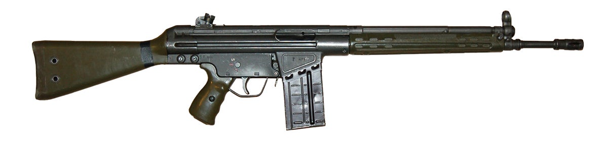
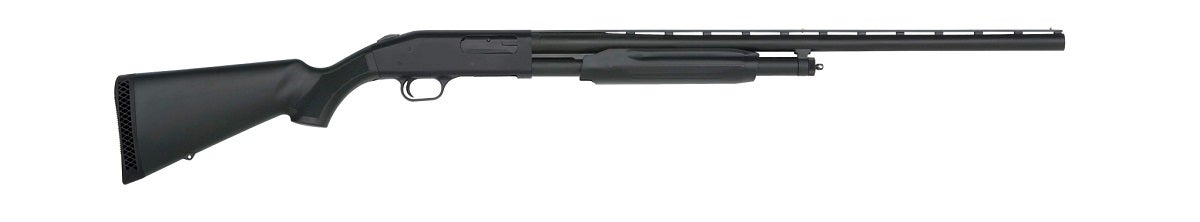
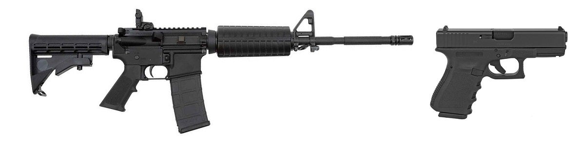
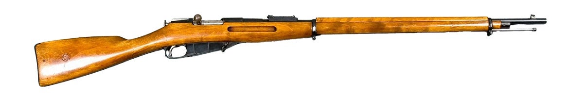
 Just as it is with power tools, each type of firearm has its own purpose. With the modularity of platforms like the AR-15, one type of gun can be configured in many different ways, covering different kinds of tasks. In my personal collection, I have a shorty AR for close range, a standard 16” do-it-all […]