Data Preprocessing
https://ift.tt/38ij8Cz
Introduction
Data preprocessing is a technique that is used to transform raw data into an understandable format. Raw data often contains numerous errors (lacking attribute values or certain attributes or only containing aggregate data) and lacks consistency (containing discrepancies in the code) and completeness. This is where data preprocessing comes into the picture and provides a proven method of resolving such issues.
Data Preprocessing is that step in Machine Learning in which the data is transformed, or encoded so that the machine can easily read and parse it. In simple terms, the data features can be easily interpreted by the algorithm after undergoing data preprocessing.
Steps involved in Data Preprocessing in Machine Learning
When it comes to Machine Learning, data preprocessing involves the following six steps:
- Importing necessary libraries.
- Importing the data-set.
- Checking and handling the missing values.
- Encoding Categorical Data.
- Splitting the data-set into Training and Test Set.
- Feature Scaling.
Let us dive deep into each step one by one.
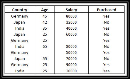
 Note: The data-set that we will be using throughout this tutorial is as listed below.
❖ Importing Necessary Libraries
Python has a list of amazing libraries and modules which help us in the data preprocessing process. Therefore in order to implement data preprocessing the first and foremost step is to import the necessary/required libraries.
The libraries that we will be using in this tutorial are:
NumPy is a Python library that allows you to perform numerical calculations. Think about linear algebra in school (or university) – NumPy is the Python library for it. It’s about matrices and vectors – and doing operations on top of them. At the heart of NumPy is a basic data type, called NumPy array.
To learn more about the Numpy library please refer to our tutorial here.
The Pandas library is the fundamental high-level building block for performing practical and real-world data analysis in Python. The Pandas library will not only allow us to import the data sets but also create the matrix of features and the dependent variable vector.
You can refer to our playlist here which has numerous tutorials on the Pandas libraries.
The Matplotlib library allows us to plot some awesome charts which is a major requirement in Machine Learning. We have an entire list of tutorials on the Matplotlib library.
Please have a look at this link if you want to dive deep into the Matplotlib library.
So, let us have a look at how we can import these libraries in the code given below:
import numpy as np
import pandas as pd
import matplotlib.pyplot as plt
❖ Importing The Dataset
Once we have successfully imported all the required libraries, we then need to import the required dataset. For this purpose, we will be using the pandas library.
Note:
- DataFrames are two-dimensional data objects. You can think of them as tables with rows and columns that contain data.
- The matrix of features is used to describe the list of columns containing the independent variables to be processed and includes all lines in the given dataset.
- The target variable vector used to define the list of dependent variables in the existing dataset.
- iloc is an indexer for the Pandas Dataframe that is used to select rows and columns by their location/position/index.
Now let us have a look at how we can import the dataset using the concepts we learned above.
dataset = pd.read_csv('Data.csv')
x = dataset.iloc[:,:-1].values
y = dataset.iloc[:,-1].values
print(x)
print(y)
Output:
[['Germany' 45.0 80000.0]
 ['Japan' 42.0 32000.0]
 ['India' 35.0 40000.0]
 ['Japan' 25.0 60000.0]
 ['Germany' 25.0 nan]
 ['India' 65.0 80000.0]
 ['Germany' nan 50000.0]
 ['Japan' 55.0 70000.0]
 ['Germany' 25.0 90000.0]
 ['India' 25.0 20000.0]]
['Yes' 'No' 'Yes' 'No' 'Yes' 'No' 'No' 'No' 'Yes' 'Yes']
❖ Checking The Missing Values
While dealing with datasets, we often encounter missing values which might lead to incorrect deductions. Thus it is very important to handle missing values.
There are couple of ways in which we can handle the missing data.
Method 1: Delete The Particular Row Containing Null Value
This method should be used only when the dataset has lots of values which ensures that removing a single row would not affect the outcome. However, it is not suitable when the dataset is not huge or if the number of null/missing values are plenty.
Method 2: Replacing The Missing Value With The Mean, Mode, or Median
This strategy is best suited for features that have numeric data. We can simply calculate either of the mean, median, or mode of the feature and then replace the missing values with the calculated value. In our case, we will be calculating the mean to replace the missing values. Replacing the missing data with one of the above three approximations is also known as leaking the data while training.
➥ To deal with the missing values we need the help of the SimpleImputer class of the scikit-learn library.
 Note
Note
- The
fit()method takes the training data as arguments, which can be one array in the case of unsupervised learning or two arrays in the case of supervised learning. -
transform
Now that we are well versed with the necessary libraries, modules, and functions needed for handling the missing data in our data set, let us have a look at the code given below to understand how we can deal with the missing data in our example data set.
import numpy as np
import pandas as pd
import matplotlib.pyplot as plt
from sklearn.impute import SimpleImputer

dataset = pd.read_csv('Data.csv')
x = dataset.iloc[:, :-1].values
y = dataset.iloc[:, -1].values
imputer = SimpleImputer(missing_values=np.nan, strategy='mean')
imputer.fit(x[:, 1:3])
x[:, 1:3] = imputer.transform(x[:, 1:3])
print(x)
Output:
[['Germany' 45.0 80000.0]
 ['Japan' 42.0 32000.0]
 ['India' 35.0 40000.0]
 ['Japan' 25.0 60000.0]
 ['Germany' 25.0 58000.0]
 ['India' 65.0 80000.0]
 ['Germany' 38.0 50000.0]
 ['Japan' 55.0 70000.0]
 ['Germany' 25.0 90000.0]
 ['India' 25.0 20000.0]]
❖ Encoding Categorical Data
All input and output variables must be numeric in Machine Learning models since they are based on mathematical equations. Therefore, if the data contains categorical data, it must be encoded to numbers.
➥ Categorical Data represents values in the data set that are non numeric.
The three most common approaches for converting categorical variables to numerical values are:
- Ordinal Encoding
- One-Hot Encoding
- Dummy Variable Encoding
In this article we will be using the the One-Hot encoding to encode and the LabelEncoder class for encoding the categorical data.
One-Hot Encoding
One hot encoding takes a column that has categorical data and then splits the column into multiple columns. Depending on which column has what value, they are replaced by 1s and 0s.
In our example, we will get three new columns, one for each country — India, Germany, and Japan. For rows with the first column value as Germany, the ‘Germany’ column will be split into three columns such that, the first column will have ‘1’ and the other two columns will have ‘0’s. Similarly, for rows that have the first column value as India, the second column will have ‘1’ and the other two columns will have ‘0’s. And for rows that have the first column value as Japan, the third column will have ‘1’ and the other two columns will have ‘0’s.
➥ To implement One-Hot Encoding we need the help of the OneHotEncoder class of the scikit-learn libraries’ preprocessing module and the ColumnTransformer class of the compose
Label Encoding
In label encoding, we convert the non-numeric values to a number. For example, in our case, the last column consists of Yes and No values. So we can use label coding to ensure that each No is converted to 0, while each Yes is converted to 1.
Let us apply the above concepts and encode our dataset to deal with the categorical data. Please follow the code given below:
# import the necessary libraries
import numpy as np
import pandas as pd
import matplotlib.pyplot as plt
from sklearn.impute import SimpleImputer
from sklearn.model_selection import train_test_split
from sklearn.preprocessing import LabelEncoder
from sklearn.preprocessing import OneHotEncoder
from sklearn.compose import ColumnTransformer

from sklearn.preprocessing import StandardScaler

# import data set
dataset = pd.read_csv('Data.csv')
x = dataset.iloc[:, :-1].values
y = dataset.iloc[:, -1].values
imputer = SimpleImputer(missing_values=np.nan, strategy='mean')
imputer.fit(x[:, 1:3])
x[:, 1:3] = imputer.transform(x[:, 1:3])
ct = ColumnTransformer(transformers=[('encoder', OneHotEncoder(), [0])], remainder='passthrough')
x = np.array(ct.fit_transform(x))
le = LabelEncoder()
y = le.fit_transform(y)
print("Matrix of features:")
print(x)
print("Dependent Variable Vector: ")
print(y)
Output:
Matrix of features:
[[1.0 0.0 0.0 45.0 80000.0]
 [0.0 0.0 1.0 42.0 32000.0]
 [0.0 1.0 0.0 35.0 40000.0]
 [0.0 0.0 1.0 25.0 60000.0]
 [1.0 0.0 0.0 25.0 58000.0]
 [0.0 1.0 0.0 65.0 80000.0]
 [1.0 0.0 0.0 38.0 50000.0]
 [0.0 0.0 1.0 55.0 70000.0]
 [1.0 0.0 0.0 25.0 90000.0]
 [0.0 1.0 0.0 25.0 20000.0]]
Dependent Variable Vector:
[1 0 1 0 1 0 1 0 1 1]
❖ Splitting The Data-set into Training Set and Test Set
After we have dealt with the missing data and the categorical data, the next step is to split the data-set into:
- Training Set: A subset of the dataset used to train the machine learning model.
- Test Set: A subset of the dataset used to test the machine learning model.
You can slice the data-set as shown in the diagram below:
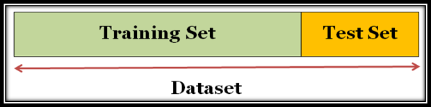
It is very important to split the data-set properly into the training set and the test set. Generally it is a good idea to split the data-set into a 80:20 ratio such that 80 percent data is in training set and 30 percent data is in test set. However, the splitting may vary according to size and shape of the data-set.
Caution: Never train on test data. For example, if we have a model that is used to predict whether an email is spam and it uses the subject, email body, and sender’s address as features and we split the dataset into training set and test set in an 80-20 split ratio then after training, the model is seen to achieve 99% precision on both, i.e. training set as well as the test set. Normally, we would expect lower precision for the test set. So, once we look at the data once again, we discover that many examples in the test set are mere duplicates of examples in the training set because we neglected the duplicate entries for the same spam email. Therefore, we cannot measure accurately, how well our model responds to new data.
Now that we are aware of the two sets that we need, let us have a look at the following code that demonstrates how we can do it:
# import the necessary libraries
import numpy as np
import pandas as pd
import matplotlib.pyplot as plt
from sklearn.impute import SimpleImputer
from sklearn.model_selection import train_test_split
from sklearn.preprocessing import LabelEncoder
from sklearn.preprocessing import OneHotEncoder
from sklearn.compose import ColumnTransformer

from sklearn.preprocessing import StandardScaler

# import data set
dataset = pd.read_csv('Data.csv')
x = dataset.iloc[:, :-1].values
y = dataset.iloc[:, -1].values
imputer = SimpleImputer(missing_values=np.nan, strategy='mean')
imputer.fit(x[:, 1:3])
x[:, 1:3] = imputer.transform(x[:, 1:3])
ct = ColumnTransformer(transformers=[('encoder', OneHotEncoder(), [0])], remainder='passthrough')
x = np.array(ct.fit_transform(x))
le = LabelEncoder()
y = le.fit_transform(y)
x_train, x_test, y_train, y_test = train_test_split(x, y, test_size=0.2, random_state=1)
print("X Training Set")
print(x_train)
print("X Test Set")
print(x_test)
print("Y Training Set")
print(y_train)
print("Y Test Set")
print(y_test)
Output:
X Training Set
[[1.0 0.0 0.0 38.0 50000.0]
 [1.0 0.0 0.0 25.0 58000.0]
 [1.0 0.0 0.0 45.0 80000.0]
 [0.0 0.0 1.0 25.0 60000.0]
 [0.0 0.0 1.0 42.0 32000.0]
 [0.0 0.0 1.0 55.0 70000.0]
 [1.0 0.0 0.0 25.0 90000.0]
 [0.0 1.0 0.0 65.0 80000.0]]
X Test Set
[[0.0 1.0 0.0 35.0 40000.0]
 [0.0 1.0 0.0 25.0 20000.0]]
Y Training Set
[1 1 1 0 0 0 1 0]
Y Test Set
[1 1]
Explaination:
train_test_split()function allows us to split the data-set into four subsets, two for the matrix of featuresxi.e.x_trainandx_testand two for the dependent variableyi.e.y_trainandy_test.x_train: matrix of features for the training data.x_test: matrix of features for testing data.y_train: Dependent variables for training data.y_test: Independent variable for testing data.
- It also contains four parameters, such that:
- the first two arguments are for the arrays of data.
test_sizeis for specifying the size of the test set.random_stateis used to fix the set a seed for a random generator in order to always get the same result.
❖ Feature Scaling
Feature scaling marks the final stage of data preprocessing. So, what is feature scaling? It is the technique to standardize or normalize the independent variables or features of the dataset in a specific range. Thus, feature scaling allows us to scale the variables in a specific range so that a particular variable does not dominate another variable.
Feature scaling can be performed in two ways:
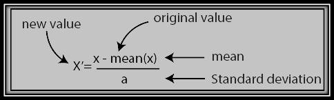
➊ Standardization
The formula for standardization is given below:
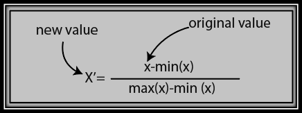
➋ Normalization
The formula for normalization is given below:
One of the most commonly asked questions among data scientists is: “Should we use Standardization or Normalization for feature scaling?”
Answer: The choice to use normalization or standardization completely depends on the problem and the algorithm being used. There are no strict rules to decide when to normalize or standardize the data.
- Normalization is good for data distribution when it does not follow a Gaussian distribution. For example, algorithms that don’t assume any distribution of the data like K-Nearest Neighbors and Neural Networks.
- Whereas, Standardization, is helpful in scenarios where the data distribution follows a Gaussian distribution. However, this is not a compulsory rule.
- Unlike, normalization, standardization has no bounding range. So, even if the data has outliers, standardization will not affect them.
In our example, we are going to use the standardization technique. Let us have a look at the following code to understand how to implement feature scaling on our dataset.
# import the necessary libraries
import numpy as np
import pandas as pd
import matplotlib.pyplot as plt
from sklearn.impute import SimpleImputer
from sklearn.model_selection import train_test_split
from sklearn.preprocessing import LabelEncoder
from sklearn.preprocessing import OneHotEncoder
from sklearn.compose import ColumnTransformer

from sklearn.preprocessing import StandardScaler

# import data set
dataset = pd.read_csv('Data.csv')
x = dataset.iloc[:, :-1].values
y = dataset.iloc[:, -1].values
imputer = SimpleImputer(missing_values=np.nan, strategy='mean')
imputer.fit(x[:, 1:3])
x[:, 1:3] = imputer.transform(x[:, 1:3])
ct = ColumnTransformer(transformers=[('encoder', OneHotEncoder(), [0])], remainder='passthrough')
x = np.array(ct.fit_transform(x))
le = LabelEncoder()
y = le.fit_transform(y)
x_train, x_test, y_train, y_test = train_test_split(x, y, test_size=0.2, random_state=1)
sc = StandardScaler()
x_train[:, 3:] = sc.fit_transform(x_train[:, 3:])
x_test[:, 3:] = sc.transform(x_test[:, 3:])
print("Feature Scaling X_train: ")
print(x_train)
print("Feature Scaling X_test")
print(x_test)
Output:
Feature Scaling X_train:
[[1.0 0.0 0.0 -0.1433148727800037 -0.8505719656856141]
 [1.0 0.0 0.0 -1.074861545850028 -0.39693358398661993]
 [1.0 0.0 0.0 0.3582871819500093 0.8505719656856141]
 [0.0 0.0 1.0 -1.074861545850028 -0.2835239885618714]
 [0.0 0.0 1.0 0.1433148727800037 -1.8712583245083512]
 [0.0 0.0 1.0 1.074861545850028 0.2835239885618714]
 [1.0 0.0 0.0 -1.074861545850028 1.4176199428093568]
 [0.0 1.0 0.0 1.7914359097500465 0.8505719656856141]]
Feature Scaling X_test
[[0.0 1.0 0.0 -0.3582871819500093 -1.4176199428093568]
 [0.0 1.0 0.0 -1.074861545850028 -2.5517158970568423]]
Explanation:
- Initially, we need to import the
StandardScalerclass of thescikit-learnlibrary using the following line of code:from sklearn.preprocessing import StandardScaler
- Then we create the object of StandardScaler class.
sc = StandardScaler()
- After that, we fit and transform the training dataset using the following code:
x_train[:, 3:] = sc.fit_transform(x_train[:, 3:])
- Finally, we transform the test dataset using the following code:
x_test[:, 3:] = sc.transform(x_train[:, 3:])
Conclusion
Congratulations! You now have all the tools in your arsenal to perform data preprocessing. Please subscribe and stay tuned for the next section of our Machine Learning tutorial!
Where to Go From Here?
Enough theory, let’s get some practice!
To become successful in coding, you need to get out there and solve real problems for real people. That’s how you can become a six-figure earner easily. And that’s how you polish the skills you really need in practice. After all, what’s the use of learning theory that nobody ever needs?
Practice projects is how you sharpen your saw in coding!
Do you want to become a code master by focusing on practical code projects that actually earn you money and solve problems for people?
Then become a Python freelance developer! It’s the best way of approaching the task of improving your Python skills—even if you are a complete beginner.
Join my free webinar “How to Build Your High-Income Skill Python” and watch how I grew my coding business online and how you can, too—from the comfort of your own home.
The post Data Preprocessing first appeared on Finxter.
Python
via Finxter https://ift.tt/2HRc2LV
December 18, 2020 at 05:57PM