I participated (just a bit) in the writing of this book as technical reviewer with Vadim and Fipar. I really enjoyed that role of carefully reading the early drafts of the chapters Daniel was writing.
Although Daniel says the book is not for the experts, I think even experts will enjoy it because several key InnoDB concepts are also covered. You can see that I refer to the book often in my A graph a day, keeps the doctor away ! series on monitoring and trending.
If you’re looking for information on transaction isolation and undo logs, fuzzy checkpointing, etc… you’ll find valuable information in the book.
The book is also enhanced with detailed illustrations that help in understanding complicated concepts (InnoDB page flushing, page 216, Source to Replica , page 235, MVCC and undo logs, page 277 are some examples).
Personally, I use this book as I used the 2nd and 3rd editions of High Performance MySQL.
From the beginning to the end of the book, Daniel focuses on the most important and measurable metric for all database consumers: query response time.
I had the chance to meet again Daniel at Percona Live and offered me a signed copy 😉
the wonderful signature 😀
I also had the privilege of having my review published in the back of the book:
If you are looking for a book to improve your knowledge of MySQL or if you are a software engineer who needs to deal with MySQL, this is a good choice.
I also recommend reading Daniel’s blog which is a complement to the book.
Not only does Lego’s Optimus Prime look great in robot mode, he actually looks even better as a truck. The transformation process very closely matches the same steps used for Hasbro’s original ‘80s toy, with the addition of a 180-degree twist at the waist, hands that fold out of the way instead of needing to be removed, and the front of the truck temporarily swinging up and out of the way providing extra clearance as various parts move around.
I like that Prime’s legs feature clips on the inside so that they can be secured together when flipped 90 degrees to form the back of the truck, and I kind of wish the arms had a similar locking mechanism too, as they tended to sag in truck mode, creating noticeable gaps in the body panels.
Photo: Andrew Liszewski – io9
I’m going to award some bonus points here because while accessories like the jetpack, axe, and energon cube don’t really have any place to call home when they’re not in use, the truck mode’s design includes a spot between Prime’s legs where his blaster can be stored more or less out of sight: a clever solution until Lego decides to release a buildable trailer for Optimus as well. (Please… pleeeeease!)
Home defense is a hot topic in the firearms community, with newbies and seasoned pros debating the merits of different platforms.
But what should you consider when setting up a home defense or bedside gun?
What happens when things go bump in the night?
Well, I’m here to help. I’m going to try and dial in on some suggestions of things I would consider essential in home defense, as well as looking at the stats behind home invasions.
I will preface this by saying that everything contained in this article is meant as a general picture and in no way should be construed as an all-inclusive, gospel, or a cookie-cutter response to fit every person or scenario.
Vaultek MXi
There are simply too many variables to account for in one article in dealing with a home defense scenario and what the correct tool for the job is.
But I’ve done my best to offer a broad perspective that should at least get you started. So keep reading to learn more!
Table of Contents
Loading…
Science of Home Defense
One of the common misconceptions in the firearms community is that we must prepare to fight off waves of invaders in a home defense situation.
Could that happen? Sure. Is it likely? Reading through recent home invasion stories reported to the police, no.
Probably not going to be fighting these off. (Photo: Rogue Pictures)
Local statistics in Las Vegas are that the likelihood is one or two (average was 1.5) persons will attempt to gain entry, though more are possibly outside in supporting roles.
This can vary from area to area, but lower-income locations typically see more burglaries and attempts.
Per the FBI’s Criminal Justice Information Services Division, a break-in occurs once every 26 seconds in the United States.
Ominous Shadow
Of those break-ins, 61% of offenders were unarmed at the time of the offense, and only 12% of all violent break-ins involved the offender having a firearm. Often, the offenders were known to the victims, and an assault occurred in only 5% of the break-ins reported.
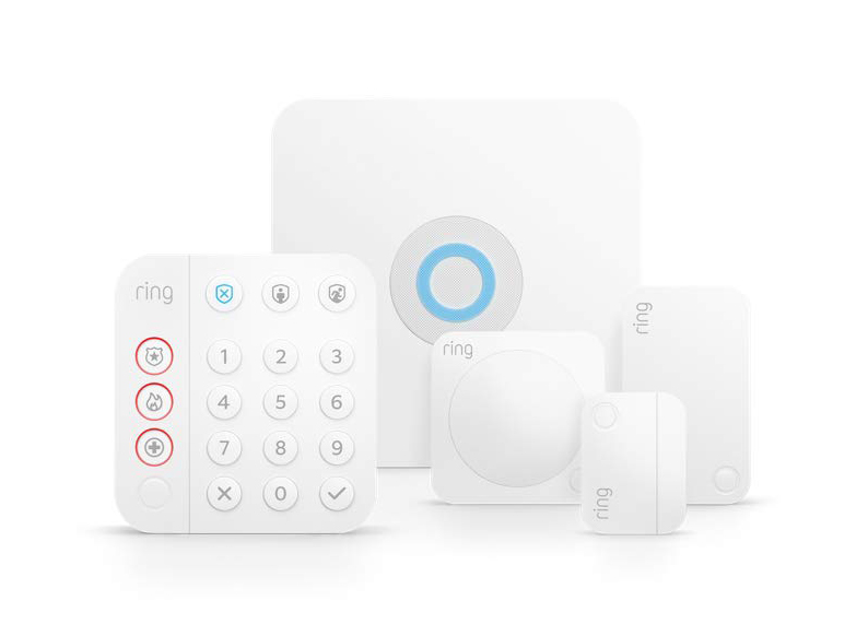
So, what does all that have to do with setting up your home defense? First and foremost, the best deterrent you can have to prevent a home invasion is a security system — 83% of would-be burglars check for some sort of security system before breaking in.
Ring Security System
If you choose to defend yourself, your home, and your family with a firearm, you need to understand that you may know the person attempting to break in, they may or may not be armed, and that the likelihood is that they want to get in and get out with cash or goods, not hurt you.
In short, make sure you understand your local laws VERY well.
What’s the Best Home Defense Tool?
This is a very complicated answer, and there isn’t a blanket “this works best for everyone” response.
Instead of going into a nuanced answer, I’m going to attempt to give some information that will highlight the strengths and weaknesses of different firearms for home defense.
Ultimately you will have to decide what will work best based on your level of familiarity and comfort with a particular platform, the layout of your house, availability of defensive ammo, and many other variables.
Why does the layout of your house matter? Defending a one-bedroom apartment will be a vastly different scenario than trying to defend a 10,000-square-foot ranch house on 27 acres of land.
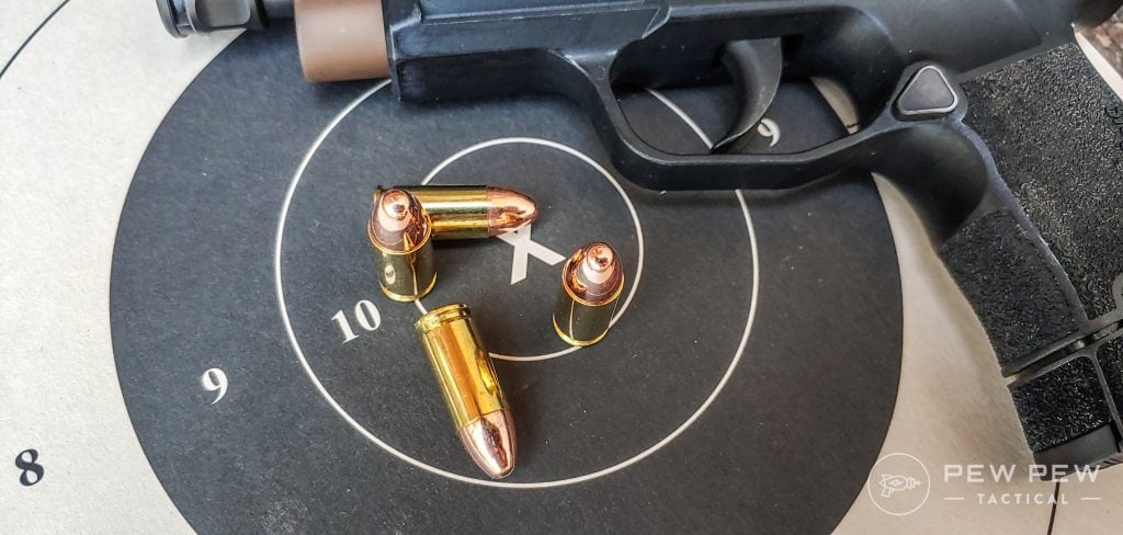
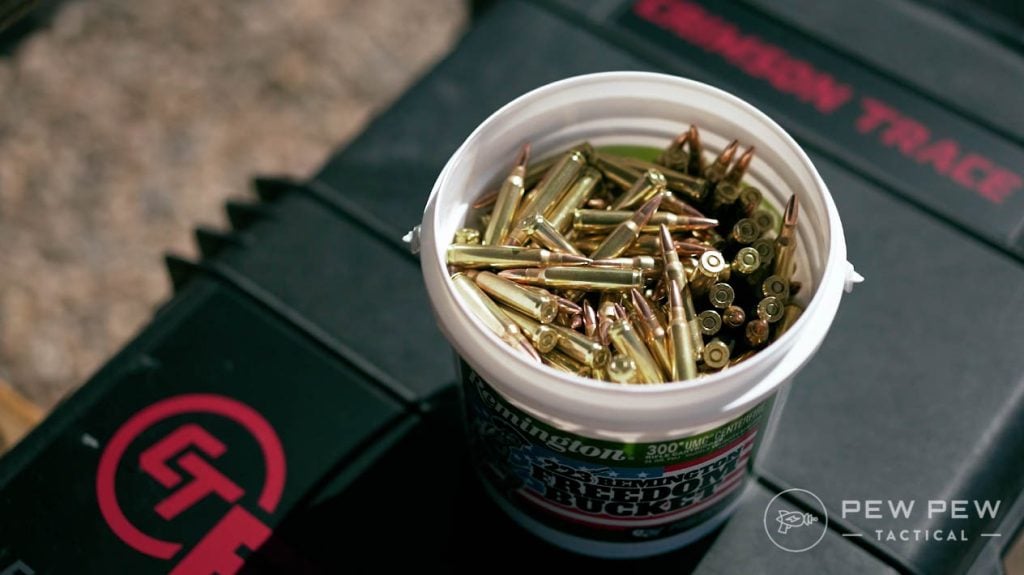
The key here is realizing that you are legally responsible for everything a bullet does once it exits the muzzle of your firearm after being discharged.
You are responsible for every one of these that leaves the barrel…
Sending a round through a wall into your neighboring townhouse means you are responsible for any damages or injuries it causes. Different tools will excel in different environments, so figure out what will do the best for you.
Investing in some deterrents can often prevent the need to use force.
We already saw that potential burglars check for a security system, so that is the first thing you should be investing in. (Or take a look at our article on the Best Ways to Secure Your Home for more tips!)
Beyond that, what’s the next step to deterring a burglary without escalating to force? A good-quality handheld flashlight and properly using it.
Let’s face facts; if something goes bump in the night, most of the time, there isn’t a need to point a gun at it.
The use of a flashlight to investigate what is skulking around your property allows you to make an informed decision on whether the use of force is necessary or if you simply caught your teenage kid sneaking back into the house.
A little light goes a long way.
If you spot a would-be burglar, the threat of being caught and detained statistically shows they are less likely to stay.
In that 5% of break-ins that turn into an assault, however, use of force may be needed, and that is where other tools are more suitable for the job.
Hands & Home Defense
I’m not getting into a debate over semi-automatic vs. revolver or a debate on which caliber is the best.
The correct answer is finding a gun that you will train to become more proficient with, that can add the features you work best with, and ensure you are confident in its use.
If you can wield a revolver well, then rock on, my friends.
I will not recommend a .22 LR as a defensive handgun, but if that is all you have, you better make it work for you.
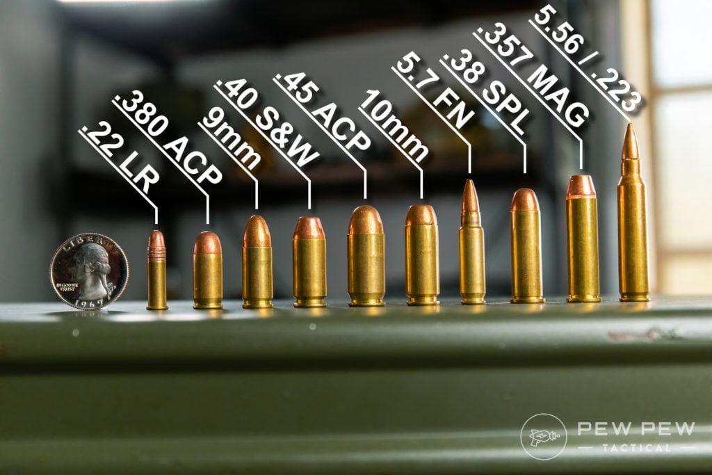
Generally, any caliber from .380 and up that offers hollow-point rounds can be suitable for a defensive gun. Each caliber will have some advantages and disadvantages.
Popular Pistol Calibers
Quality matters for defensive guns. Right now, finding quality guns can be both difficult and expensive, but you have to ask yourself what your life is worth.
Let’s face it, in the middle of the night; you should have the advantage in your home over a stranger. You know the layout better, you know where obstacles typically are, and you are just generally more familiar. Why not press that advantage with your firearm?
You know the layout better than they do.
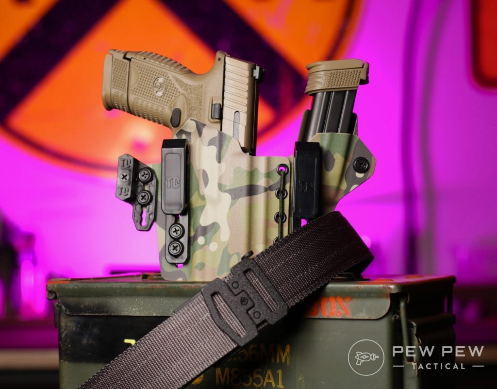
If you find yourself in a dark house trying to defend yourself, getting positive target identification and getting sights on target are the two things with which you need to be concerned — speaking in terms of operating the gun itself, not considering things like finding and using cover, etc.
To this end, I do recommend a weapon-mounted light of good quality — Streamlight, Surefire, Modlite, etc.
1911s with Lights & Lasers
Additionally, I am a huge advocate for adding an optic to your pistol. Optics allow you to be threat-focused, rather than requiring you to switch to sight focus beyond a certain distance.
Optics allow you to acquire your aiming device regardless of lighting conditions and permit faster follow-up shots with more consistency, regardless of shooting experience.
Bunch of Micro Guns and Red Dots
Can’t night sights/fiber optic sights do the same thing? Yes and no. They will allow you to find your sights faster, but you are still limited by lighting conditions to get sights on target, and iron sights still require sight focus vs. being target focused.
The last component is ammo. Find good quality, consistent hollow points that will get the job done.
Popular 9mm Ammo
Examples of this would include but are not limited to Speer Gold Dot, Hornady Critical Duty, or Federal HST for larger handguns like the Glock G17 and G19.
For shorter barreled guns like Glock G43x, S&W Shield, or Sig P365, Hornady Critical Defense or Federal Punch are better options.
Speaking with Chuck Haggard of Agile/Training & Consulting, he mentioned that shorter barreled handguns lead to the round not fully expanding on some of the duty grade hollow points.
His testing and experience showed that Critical Defense was a much better choice in that scenario.
Glock G43X
Make sure your gun is rated for any +P or +P+ ammo you intend to shoot, and then shoot a magazine worth through your gun to make sure it cycles without any issue.
Pistols do have their limits, and you need to know them.
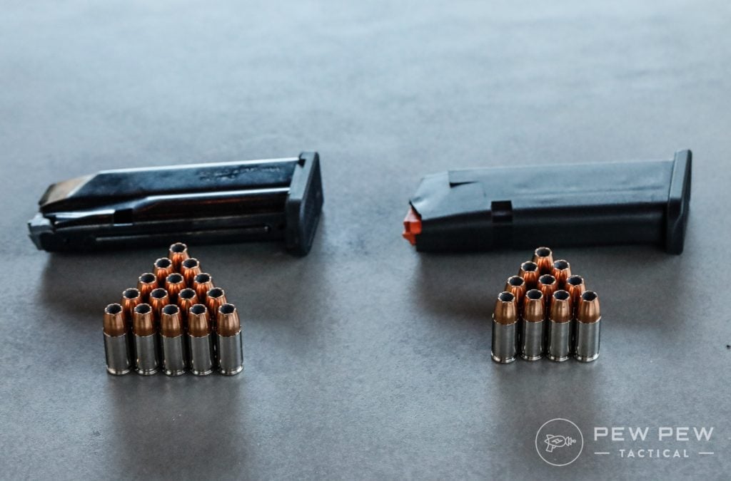
Depending on the handgun you’ve selected, you will have between six and 17 rounds to use for your defense without reloading.
Shield vs Stock Glock 43x Mag
Looking back at the average number of attackers, that is between three and eight shots at each adversary.
Add in adrenaline and the high stress of the situation, and you now have a scenario where you are likely reverting to your lowest proficiency and training to put hits on target.
Rifles for Home Defense
Many, myself included, choose to use a rifle or pistol version of a rifle for home defense.
Rifles offer a more stable, more forgiving firing platform than handguns due to the increased points of body contact with the gun.
Additionally, they typically offer more ammunition to feed and, in most cases, provide increased velocity over handguns.
So, when will a rifle be an advantage over a handgun? If your house is laid out in such a manner that you can create distance, a rifle is going to generally be better than a handgun.
I want to clarify this in that shot placement matters; either way, people can generally fire a rifle better than a handgun at low skill levels. At 15 to 20 yards, both can be effective; it will come down to training and comfort.
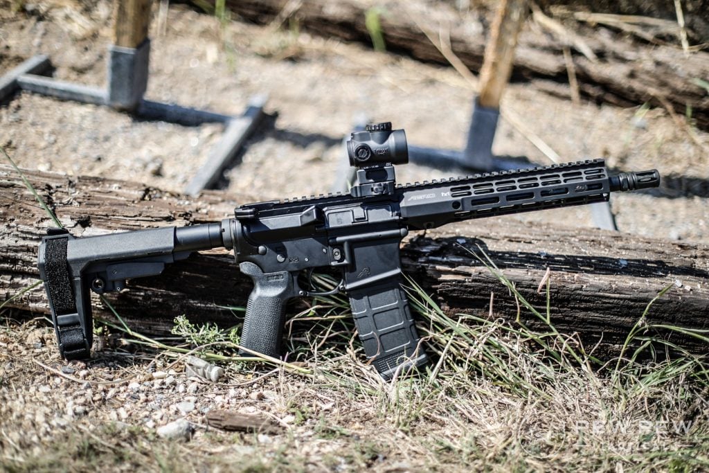
Aero AR-15 10.5″ Pistol
In my case, my entire family is housed on the second floor of our home. I can then use a rifle to defend against people coming upstairs and know that it will be effective.
Just like with handguns, a rifle will benefit from a weapon-mounted light. Target identification is still a priority, even more so at greater distances.
Cloud Defensive OWL
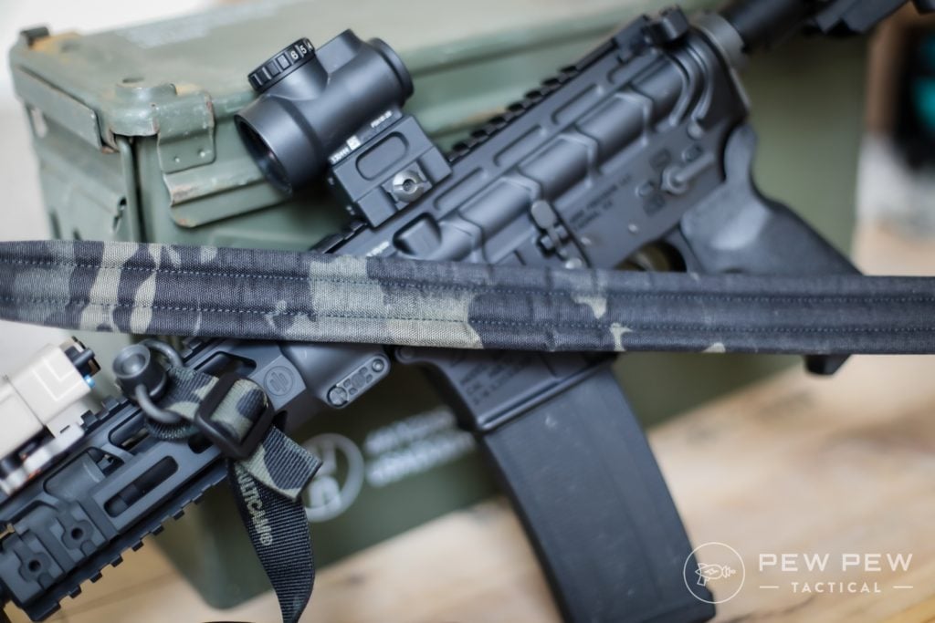
Some form of quality optic is needed as well. I prefer red dots that I can leave on like an Aimpoint CompM5 or T2 so that my gun is ready when I pick it up. I know others that run low-power variable scopes and are very effective.
I would avoid using just iron sights, as you still suffer the same limitations as handgun sights. Invest in a quality optic, stay away from knocks-offs and low-quality products, and prosper.
Faxon Firearms Ascent
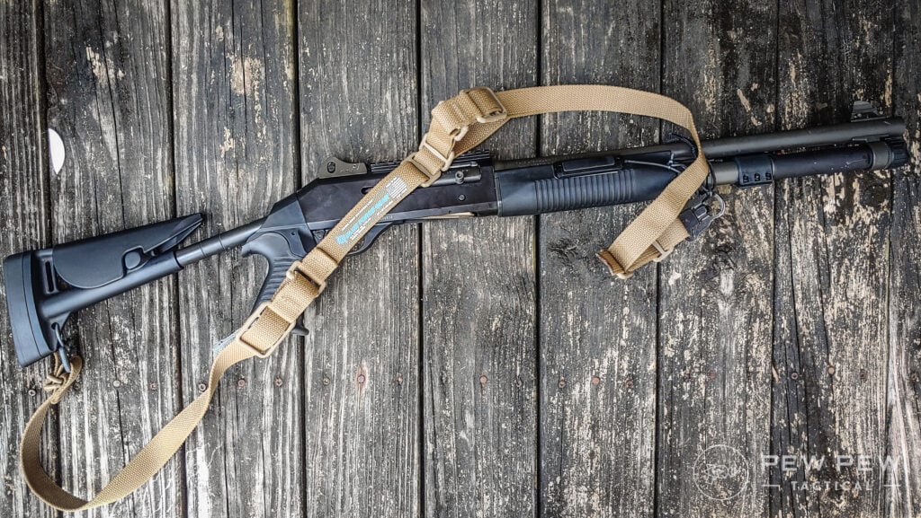
Lastly, a sling is a must-have for a defensive rifle. This allows the user to retain possession of the weapon if hand to hand occurs and allows for retention of the rifle if you need your hands free to pick something or someone up to help.
Rifles are not without their drawbacks, though. That sling that I just mentioned means that the gun is attached to you to some extent. A knowledgeable attacker can use that as leverage against you to control your body and/or throw you.
Pew Pew Tactical Sling
In closer quarters or houses with lots of turns, a longer barrel can be a hindrance in terms of maneuverability.
Ammo selection, along with good shot placement, also plays a huge role in the effectiveness of a rifle. Once again, something like Speer Gold Dot, Federal LE Tactical, or Hornady TAP FDP that are made to have a hollow or soft point allow for better defensive use than a full metal jacket round.
TAP and other fragmenting rounds are especially worth considering if over-penetration is a concern in smaller living spaces. Please understand that fragmenting rounds are different than frangible rounds, and under no circumstances are frangible rounds a go-to for personal protection.
Going back to our average number of people in the break-in, rifles offer more rounds to put on target.
An AR-15 magazine comes in 10-round, 20-round, and 30-round magazines as the most common options. You can get larger capacity drum magazines, but many tend to be lower quality, finicky, and not reliable to consider for a self-defense scenario.
All the mags
As I mentioned above, it may take more than one round to stop someone from attacking you, so having more ammunition to expend in that pursuit is a good thing.
Shotgun Setups for Home Defense
Shotguns for home defense use have become a more heated topic in the last few years.
Search any gun forum or message board, and you’ll encounter people saying…shotguns are the best defensive gun ever, you just need to rack the action to scare away every bad guy in a 3-mile radius, you don’t have to aim, etc.
The truth is that shotguns have their place in home defense, but like anything else, they aren’t a blanket answer to a problem. Sometimes shotguns will be the optimal choice and other times they won’t.
Once you have a good-quality, reliable shotgun, the next step is patterning your ammo.
This involves getting the ammo you intend to use and shooting it at various distances to see how the pellets spread and pattern on a target.
Practicing at the range with your ammo will give you a good idea of how it flies
This is important, as using different types of buckshot with different guns will get you different results. As you are responsible for everything your ammo does after it is fired, you need to know exactly where these pellets will fly, where they end up, and if you will face any unintended damage.
There are two viable shotgun rounds for defense, buckshot, and slugs. Birdshot and snakeshot are not suitable for self-defense, and their use could leave you facing an angry opponent that is still able to function.
12ga Birdshot, Opened
Buckshot utilizes larger pellets that are ideally suited for home defense, but not all of them pattern the same. Depending on your barrel and if you are running a choke or not, Federal Flight Control may be an option, and generally, 8-pellet buckshot is going to be superior to 9-pellet.
Federal FliteControl shell, dissected 2
Slugs are your other option for self-defense. Slugs utilize a solid projectile instead of pellets and were originally designed for use on larger game.
Think of firing a softball instead of marbles. Slugs will be a better choice for defensive rounds at longer distances, as buckshot patterns will spread out more there. Inside of 10 yards, though, buckshot will be better.
12ga Slug, Opened
Distance is generally going to be the enemy of a shotgun beyond 30 yards or so. Inside of that range, a shotgun is a devastating tool that will very quickly end engagements.
Contrary to popular myth, you still have to aim a shotgun for it to be effective. To that end, a good quality light for target identification is worth considering. As with other platforms, mounting an optic is not a bad idea.
Blue Force Gear Vickers Sling
Additionally, a sling is a great idea for the same reason discussed earlier. Also, keep in mind that a shotgun will generally be longer and often heavier than an AR-15 or AK-47.
Shotguns do have their drawbacks, though. Like rifles, movement and mobility can be hindered by the size of the gun.
Additionally, recoil mitigation for follow-up shots is something that must be trained, as some people will find the gun awkward and uncomfortable without adjustments made.
Mossberg Retrograde 590A1
Reloading a shotgun is also a bit more involved than slapping a fresh magazine in, so it is a skill that must be trained to be fast and proficient at it.
Applying shotguns to our two-attacker scenario, this is where things are very different.
Depending on which shotgun model you have, the tube may hold between six and eight rounds without extended tubes.
While this leaves only three or four rounds per assailant within a shotgun’s effective range, one round delivered to an attacker is devastating. The shot must still hit, but if it does, there is a very high probability that the fight is now over and your opponent’s behavior has changed.
Final Thoughts
No two scenarios are the same, and thus no answer will fit universally. Find the self-defense setup that makes sense for you, train with the tools and understand the tactics needed to win the fight.
Also, source out quality information, and do not be afraid to challenge the misconceptions you might have or might have heard.
In the end, defending yourself and those you care about is the only thing that matters, so give yourself as much advantage as possible.
In today’s world, it’s difficult to find unbiased news and get a true sense of what’s going on around you. This applies to widespread topics, like politics or science, as well as more personalized topics, like gaming, sports, or film.
Luckily, you don’t have to scour individual news sites anymore. There are apps dedicated to collecting news from different sources, making it easy for you to keep up with everything you’re interested in and get different viewpoints. Flipboard and Feedly are two of the most popular apps for keeping track of new info, but which is better? Let’s check it out!
Download: Feedly for Android | iOS (Free, in-app purchases available)
User Interface
Overall, Flipboard has a more intuitive user interface that seems more fleshed out for the average, everyday user when compared to Feedly.
Articles and topics of interest are displayed with a large square image that’s more aesthetically pleasing. Flipboard also lets you flip through content on the home screen, similar to the flipping motion of reading an actual magazine.
There’s nothing overly special about Feedly’s user interface. It’s straightforward and fairly easy to use, but a little boring, at least compared to Flipboard. When you see articles on the home screen, there’s less of a focus on the featured image for the article.
MAKEUSEOF VIDEO OF THE DAY
Instead, the article title is bolded, there’s sometimes a brief sentence displayed under the title, and then there’s a small image to the right.
Navigating the News
When you first download Flipboard and set up your account, you’ll be asked to select a variety of hashtags based on what your interests are. You can select as many as you want to, but you have to select at least three.
Then, your home page, or pages, are personalized to the content you’re interested in seeing. You can flip through content on the home page, or head over to your Following tab to see articles with specific hashtags you follow. Being able to navigate the news this way within the Flipboard app makes it much more easily personalized than what Feedly offers.
Feedly does a good job of displaying popular news stories that interest you on the home screen, but you have to do a lot of work behind the scenes to get your home screen looking the way you want it. Whereas Flipboard allows you to add topics by hashtags, Feedly lets you favorite or follow specific websites within a niche.
For example, if you’re interested in keeping up with the latest gaming news, you could search that topic and find multiple sites related to that industry. Then, you need to personally select the sites that you want to read stories from to fill your feed.
If you don’t feel like putting in all the effort to personalize your feed, you can browse through the Explore tab to read some of the most popular stories. Since you browse news by the sites you choose to follow, it’s a bit harder to find fair and balanced news on Feedly than it is on Flipboard.
Sharing the News
Both apps let you share articles on almost every platform you can think of. Want to send a quick link to your mom with a recipe you think she’ll like? Or send the latest sports news to a friend to see what they thought of the game last night?
On Flipboard, when you open an article and tap the share button, you’ll see a list of all your sharing-compatible apps pop up. Select an app and it’ll share the article title and a shortened link.
When you tap the share button on Feedly, you’ll see your most recent or most popular apps show up to quickly share the article. You can, of course, always scroll to the end to view others, but they’re not readily displayed like in the Flipboard app.
Saving Articles For Later
It’s not always possible to read every story that piques your interest as soon as you see it. Luckily, both Flipboard and Feedly allow you to save stories to read them when you find time. You can also use this feature to bookmark articles you want to save for the future or eventually show to a family member or friend.
Flipboard lets you organize articles into your own personal “magazines.” You can customize the titles of your magazines to make it easy to find articles later, as well as reset the cover image to reflect the last article you added.
You can add as many magazines as you want. If you select the Profile tab all the way to the right on the bottom navigation bar, you’ll see all your magazines displayed how you have them organized. By tapping and holding a magazine cover, you can drag it around the screen to reorder it.
You can create magazines simply for collecting and saving stories for you or your followers, for sharing among friends and family, or for mixing together content from Twitter feeds, blogs, and other news sources.
While Flipboard allows you to create custom magazines in addition to a “Save For Later” magazine, the Feedly app only lets you bookmark articles to read later. There’s no way to organize the articles you save. Instead, everything is saved in one long list.
You can change what the article looks like in this list, like a card with a picture, a magazine list, or just text from the article. But you can’t organize articles by topic or create a separate section for recipes, as an example, that you can simply save forever.
Once you’ve read an article that you saved to read later, you can remove the bookmark to take it off your reading list instantly. Or, you can read through all the articles on your list and then mark all of them as read at once.
Finding Reputable News Shouldn’t Be Difficult
Both Flipboard and Feedly make it easy for users to find news on topics that interest them, whether you want to find out what’s going on in other countries or what’s going on in the industry you work in. With such a variety of sources, it’s easy to find balanced stories that offer different opinions on even the most controversial topics.
With either app, you can collect news relevant to you instead of always perusing a single site to find your news.
Browsing an individual site almost always means skipping over stories that just don’t interest you, but by using a personalized app, everything you see will be based on your interests! Between Flipboard and Feedly, I’d say Flipboard is the better news app because it’s more personalized and easier to use.
There are two types of IFs in MySQL: the IF statement and the IF function. Both are different from each other. In this article, we will explain their diversities and show usage examples. Also, we will review other MySQL functions. Contents MySQL IF statements MySQL IF-THEN statement MySQL IF-THEN-ELSE statement MySQL IF-THEN-ELSEIF-ELSE statement Examples of […]
I am a big fan of Percona Monitoring and Management (PMM) and am happy to report that setting up Percona Platform is as easy to set up and offers a lot of value. Percona Platform reached GA status recently and I think you will find it a handy addition to your infrastructure.
What is Percona Platform?
Percona Platform brings together enterprise-level distributions of MySQL, PostgreSQL, and MongoDB plus it includes a range of open source tools for data backup, availability, and management. The core is PMM which provides database management, monitoring, and automated insights, making it easier to manage database deployments. The number of sites with more than 100 separate databases has grown rapidly in the past few years. Being able to have command and control of that many instances from a CLI has become impossible. Businesses need to move faster in increasingly complex environments which puts ever-increasing pressure on database administrators, developers, and everyone involved in database operations. The spiraling levels of demand make it harder to support, manage, and correct issues in database environments.
What Percona Platform provides is a unified view of the health of your entire database environment to quickly visually identify and remediate issues. Developers can now self-service many of their database demands quickly and efficiently so they can easily provision and manage databases on a self-service basis across test and production instances. So you spend fewer resources and time on the management of database complexity.
The two keys to Percona Platform are Query Analytics (QAN), which provides granular insights into database behavior and helps uncover new database performance patterns for in-depth troubleshooting and performance optimization, and Percona Advisors, which are automated insights, created by Percona Experts to identify important issues for remediation such as security vulnerabilities, misconfigurations, performance problems, policy compliance, and database design issues. Automated insights within Percona Monitoring and Management ensure your database performs at its best. The Advisors check for replication inconsistencies, durability issues, password-less users, insecure connections, unstable OS configuration, and search for available performance improvements among other functions.
Percona Platform is a point of control for your database infrastructure and augments PMM to be even more intelligent when connected to the Percona Platform. By connecting PMM with the Percona Platform, you get more advanced Advisors, centralized user account management, access to support tickets, private Database as a Service, Percona Expertise with the fastest SLAs, and more.
So How Do I Install Percona Platform?
The first step is to install PMM by following the Quick Start Guide. You need version 2.2.7 or later.
Third, you will need to connect that account to PMM.
I will assume that you will already have PMM installed. Did I mention that PMM is free, open source software?
The signup form allows you to create a new account or use an existing account.
Now you can create a name for your organization.
After creating your username and password, create your organization
Now login to your PMM dashboard and select the Settings / Percona Platform. You will need to get your ‘Public Address’ which the browser can populate the value for you if need be.
The PMM Server ID is automatically generated by PMM. You will need to provide a name for your server, and you will need a second browser window to login into Percona Platform to get the Percona Platform Access Token (this token has a thirty-minute lifetime, so be quick or regenerate another token).
Go back into PMM, paste the Access Token into the Percona Platform Access Token field, and click Connect.
On the Percona Platform page, you will see your PMM instances. Congratulations, you are using Percona Platform!
Advisor Checks
All checks are hosted on Percona Platform. PMM Server automatically downloads them from here when the Advisors and Telemetry options are enabled in PMM under Configuration > Settings > Advanced Settings. Both options are enabled by default.
Depending on the entitlements available for your Percona Account, the set of advisor checks that PMM can download from Percona Platform differ in terms of complexity and functionality.
If your PMM instance is not connected to Percona Platform, PMM can only download the basic set of Anonymous advisor checks. As soon as you connect your PMM instance to Percona Platform, has access to additional checks, available only for Registered PMM instances.
If you are a Percona customer with a Percona Customer Portal account, you also get access to Paid checks, which offer more advanced database health information. A list is provided below.
Check Name
Description
Tier
MongoDB Active vs Available Connections
Checks the ratio between Active and Available connections.
Registered, Paid
MongoDB Authentication
Warns if MongoDB authentication is disabled.
Anonymous, Registered, Paid
MongoDB Security AuthMech
Warns if MongoDB is not using the default SHA-256 hashing as SCRAM authentication method.
Paid
MongoDB IP Bindings
Warns if MongoDB network binding is not set as recommended.
Anonymous, Registered, Paid
MongoDB CVE Version
Shows an error if MongoDB or Percona Server for MongoDB version is not the latest one with CVE fixes.
Anonymous, Registered, Paid
MongoDB Journal Check
Warns if journal is disabled.
Registered, Paid
MongoDB Localhost Authentication Bypass is Enabled
Warns if MongoDB localhost bypass is enabled.
Anonymous, Registered, Paid
MongoDB Non-Default Log Level
Warns if MongoDB is not using the default log level.
Paid
MongoDB Profiling Level
Warns when the MongoDB profile level is set to collect data for all operations.
Registered, Paid
MongoDB Read Tickets
Warns if MongoDB is using more than 128 read tickets.
Paid
MongoDB Replica Set Topology
Warns if the Replica Set cluster has less than three members.
Registered, Paid
MongoDB Version
Warns if MongoDB or Percona Server for MongoDB version is not the latest one.
Anonymous, Registered, Paid
MongoDB Write Tickets
Warns if MongoDB network is using more than 128 write tickets.
Paid
Check if Binaries are 32-bits
Notifies if version_compatible_machine equals i686.
Anonymous, Registered, Paid
MySQL Automatic User Expired Password
Notifies if version_compatible_machine equals i686.
Registered, Paid
MySQL InnoDB flush method and File Format check
Checks the following settings: innodb_file_format, innodb_file_format_max, innodb_flush_method and innodb_data_file_path
Registered, Paid
MySQL Checks based on values of MySQL configuration variables
Checks the following settings: innodb_file_format,innodb_file_format_max,innodb_flush_method and innodb_data_file_path.
Paid
MySQL Binary Logs checks, Local infile and SQL Mode checks
Warns about non-optimal settings for Binary Log, Local Infile and SQL mode.
Registered, Paid
MySQL Configuration Check
Warns if parameters are not following Percona best practices, for infile, replication threads, and replica checksum.
Paid
MySQL Users With Granted Public Networks Access
Notifies about MySQL accounts allowed to be connected from public networks.
Registered, Paid
MySQL User Check
Runs a high-level check on user setup
Registered, Paid
MySQL Advanced User Check
Runs a detailed check on user setup
Paid
MySQL Security Check
Runs a detailed check on user setup
Paid
MySQL Test Database
This check returns a notice if there is a database with name ‘test’ or ‘test_%’.
Registered, Paid
MySQL Version
Warns if MySQL, Percona Server for MySQL, or MariaDB version is not the latest one.
Anonymous, Registered, Paid
PostgreSQL Archiver is Failing
Verifies if the archiver has failed.
Paid
PostgreSQL Cache Hit Ratio
Checks database hit ratio and complains when this is too low.


 A critical skill for any rifle shooter, mounting your own scope will save you time, money, and teach a core skill for long range shooting.Recoil


