Category: Uncategorized

-- Every hot-path query carries customer_id, so it routes to one shard.
SELECT * FROM orders
WHERE customer_id = 88213        -- shard key: single-shard lookup
  AND status = 'shipped'
ORDER BY created_at DESC;

The trade-off to accept consciously is that cross-shard-key queries become expensive. Analytics that aggregate across all customers, admin searches by email, or reports spanning every tenant cannot be answered from a single shard. The pattern is not to avoid these but to serve them differently: route analytical queries to a separate columnar store or data warehouse, maintain secondary lookup tables for the few alternate access paths you truly need, and accept that the operational database is optimized for its dominant access pattern, not every possible one.

Even if you are not sharding today, choosing and consistently populating a shard key now means that when you do shard, it is a routing change rather than a schema migration across billions of rows.

Pattern 3: Denormalize Deliberately to Kill the Join Fan-Out

Normalization is the right default. It prevents update anomalies and keeps each fact in exactly one place. But the relational join—the mechanism that makes normalization work—is precisely the operation that does not partition cleanly. A join between two tables on different shard keys forces a cross-shard operation. Even on a single server, a query that joins five tables to render one screen multiplies the work and the lock surface.

The scalability pattern is targeted denormalization: duplicate the specific fields that hot-path queries need so those queries can be answered from a single row or a single table, without joins.

The discipline here matters. Indiscriminate denormalization creates a maintenance nightmare where every update has to touch a dozen copies. The pattern is to denormalize only the fields that appear together in your highest-volume read paths, and to be explicit about which table owns the source of truth versus which holds a cached copy.

-- Instead of joining orders -> customers on every order list view,
-- store the small, slowly-changing customer fields the list needs.
CREATE TABLE orders (
    id              BIGINT UNSIGNED NOT NULL,
    customer_id     BIGINT UNSIGNED NOT NULL,
    customer_name   VARCHAR(120) NOT NULL,   -- denormalized copy
    customer_tier   TINYINT NOT NULL,        -- denormalized copy
    total_cents     INT UNSIGNED NOT NULL,
    created_at      DATETIME(3) NOT NULL,
    PRIMARY KEY (customer_id, id)
) ENGINE=InnoDB;

When the source data changes (a customer renames their account), you update the copies asynchronously—via application logic, a change-data-capture pipeline, or a background job. The key insight is that for many fields the consistency requirement is “eventually,” not “immediately,” and trading a small consistency window for join-free reads is exactly the trade that buys linear read scalability.

A common and powerful variant is the read model or materialized view table: a table whose sole purpose is to serve one expensive query shape, populated by aggregating or flattening normalized source data. The write path stays normalized; the read path gets a purpose-built, join-free table.

Pattern 4: Split Tables Vertically to Keep Hot Rows Small

InnoDB reads and writes data in 16 KB pages. The narrower your rows, the more rows fit per page, the more of your working set fits in the buffer pool, and the less I/O each query costs. A wide table—dozens of columns including large TEXT, JSON, or BLOB fields—wastes buffer pool space on data that most queries never touch.

Vertical partitioning splits one wide table into a narrow “hot” table and one or more “cold” tables, joined by the same primary key. The columns accessed on every request stay in the slim hot table; the rarely-read bulk moves to a companion table.

-- Hot table: tiny rows, queried constantly, fits entirely in memory.
CREATE TABLE users (
    id            BIGINT UNSIGNED PRIMARY KEY,
    email         VARCHAR(255) NOT NULL,
    status        TINYINT NOT NULL,
    last_login_at DATETIME(3),
    UNIQUE KEY (email)
) ENGINE=InnoDB;

-- Cold table: large, rarely-read fields kept out of the hot path.
CREATE TABLE user_profiles (
    user_id     BIGINT UNSIGNED PRIMARY KEY,
    bio         TEXT,
    preferences JSON,
    avatar_blob LONGBLOB,
    CONSTRAINT fk_profile FOREIGN KEY (user_id) REFERENCES users(id)
) ENGINE=InnoDB;

This pattern is especially valuable for tables that mix frequently-updated columns with large static ones. Updating a single counter on a row that also holds a megabyte JSON document means InnoDB may rewrite far more than the changed bytes and generate large undo and redo records. Separating volatile small columns from stable large ones reduces write amplification and replication payload, both of which directly affect how far you can scale writes.

Pattern 5: Use Native Partitioning for Time-Series and Lifecycle Data

Not all scaling is horizontal across servers. A single MySQL instance can manage far larger tables when the table is partitioned internally so that queries and maintenance touch only the relevant slice. MySQL’s native PARTITION BY RANGE on a date or sequential ID is the canonical pattern for time-series, event, and log-style data.

The benefits compound at scale. Queries with a date predicate undergo partition pruning—the optimizer skips every partition outside the range, so a query over last week’s data never scans last year’s. Equally important, dropping old data becomes instant: ALTER TABLE ... DROP PARTITION is a near-metadata-only operation, compared to a DELETE that would scan, lock, and log millions of rows and bloat the table.

CREATE TABLE events (
    id          BIGINT UNSIGNED NOT NULL,
    user_id     BIGINT UNSIGNED NOT NULL,
    event_type  VARCHAR(40) NOT NULL,
    created_at  DATETIME NOT NULL,
    PRIMARY KEY (id, created_at)          -- partition column must be in the PK
)
PARTITION BY RANGE (TO_DAYS(created_at)) (
    PARTITION p2026_05 VALUES LESS THAN (TO_DAYS('2026-06-01')),
    PARTITION p2026_06 VALUES LESS THAN (TO_DAYS('2026-07-01')),
    PARTITION p2026_07 VALUES LESS THAN (TO_DAYS('2026-08-01')),
    PARTITION pmax      VALUES LESS THAN MAXVALUE
);

Two constraints shape this pattern. The partitioning column must be part of every unique key, including the primary key—hence (id, created_at) above. And partition maintenance (adding next month’s partition, dropping the oldest) should be automated, because a partitioned table that runs out of defined ranges or accumulates unbounded partitions reintroduces the very problems it was meant to solve. Treat partition rotation as a scheduled operational job, not a one-time DDL.

Pattern 6: Eliminate Write Hotspots and Contention Points

A hotspot is any single row, page, or counter that a large fraction of writes must touch. Hotspots are the enemy of linear scaling because they serialize writes that should run in parallel—no amount of added hardware helps when everything queues behind one lock.

The most common hotspot is the global counter: a single row holding a total that every transaction increments, such as a “likes” count on a viral post or a balance on a shared account. Under load, every writer contends for the lock on that one row.

The fix is the sharded counter pattern. Instead of one row, maintain N rows and have each writer increment a randomly or hash-chosen shard. The true total is the sum across shards, computed at read time (or periodically rolled up).

CREATE TABLE post_like_counters (
    post_id   BIGINT UNSIGNED NOT NULL,
    shard     TINYINT UNSIGNED NOT NULL,    -- e.g. 0..63
    likes     BIGINT UNSIGNED NOT NULL DEFAULT 0,
    PRIMARY KEY (post_id, shard)
) ENGINE=InnoDB;

-- Writes spread across 64 rows instead of contending on one:
UPDATE post_like_counters
SET likes = likes + 1
WHERE post_id = 991 AND shard = FLOOR(RAND() * 64);

-- Reads aggregate (cache the result if needed):
SELECT SUM(likes) FROM post_like_counters WHERE post_id = 991;

Related hotspot patterns worth internalizing: prefer append-only inserts over in-place updates where the domain allows it, because inserts to ordered keys contend far less than updates to shared rows; avoid status-flag columns that the entire fleet polls and updates in lockstep; and be wary of “queue” tables where every worker hammers the same few “ready” rows—use techniques like SELECT ... FOR UPDATE SKIP LOCKED to spread workers across rows. Each of these is the same lesson: find the shared point and break it into many independent points.

Pattern 7: Index for the Working Set, Not Every Possible Query

Indexes accelerate reads but tax writes—every secondary index must be updated on insert, and in InnoDB each one carries the full primary key as its row pointer. On a write-heavy table at scale, an over-indexed schema can spend more effort maintaining indexes than storing data, capping write throughput.

The scalable approach is to index for your actual hot query shapes and prune the rest. A few principles carry most of the value:

Composite indexes should match query order. An index on (customer_id, status, created_at) serves equality-on-customer-then-status-then-range-on-date queries efficiently, following the leftmost-prefix rule. The column order should mirror how predicates are applied.

Covering indexes eliminate row lookups. If an index contains every column a query needs, InnoDB answers the query from the index alone, never touching the clustered index. For high-frequency queries, designing a covering index is one of the highest-return optimizations available.

Keep secondary indexes narrow, because every one of them stores the primary key. This is another reason fat primary keys (random UUIDs) hurt: they bloat not just the table but every index on it. A compact key keeps the whole index footprint small enough to stay in memory.

Periodically audit for unused and redundant indexes. An index that no query uses is pure write overhead. At scale, removing it can measurably lift write throughput—a rare optimization that costs nothing and helps everywhere.

Pattern 8: Model for Replication and Eventual Consistency from Day One

Linear read scaling on MySQL almost always means read replicas: a primary handles writes, and reads spread across replicas. This works beautifully—until the schema and the application assume read-your-own-writes consistency that asynchronous replication cannot guarantee.

The schema-level pattern is to make data tolerant of replication lag. Avoid designs that require reading a value immediately after writing it on a different node. Where read-after-write matters (a user updating their own profile and expecting to see the change), route those specific reads to the primary, and design the schema so that the set of such “must-be-fresh” reads is small and well-defined rather than pervasive.

This also influences how you model derived data. Counters, aggregates, and denormalized copies (Patterns 3 and 6) are naturally eventually-consistent, which fits replication well. Trying to keep them transactionally exact across replicas reintroduces coordination. Embracing eventual consistency for the data that can tolerate it is what lets the read tier scale out linearly.

A practical corollary: keep transactions short and touch as few rows as possible. Long, wide transactions hold locks longer, generate large binlog events, and widen replication lag—all of which erode the headroom replicas give you. Schema choices that naturally lead to small, focused writes (narrow hot tables, append-only patterns, sharded counters) pay off again here.

Pattern 9: Bound Every Table’s Growth

An unbounded table is a deferred outage. A table that grows forever will eventually exceed the buffer pool, then sensible index sizes, then maintenance windows, until routine operations like adding a column or rebuilding an index become multi-hour ordeals. Linear scalability assumes you can keep adding capacity; an unbounded table eventually makes each unit of capacity more expensive than the last.

The pattern is to design a retention and archival strategy into the schema itself, not bolt it on later. Time-range partitioning (Pattern 5) is the cleanest mechanism: old partitions drop instantly. For data that must be retained but not served hot, move it to cheaper archival tables or external storage on a schedule, keeping the operational table sized to the working set. Define, in writing, how large each high-growth table is allowed to get and what happens when it approaches that limit—before the table forces the answer on you at the worst possible time.

Bringing the Patterns Together

These patterns reinforce one another, and the through-line is consistent. Distribution-friendly primary keys make sharding possible. A well-chosen shard key makes the dominant queries single-shard. Deliberate denormalization and read-model tables remove the joins that would otherwise force cross-shard work. Vertical partitioning and tight indexing keep the hot working set in memory. Native partitioning and bounded growth keep individual tables fast and maintainable. Hotspot elimination and replication-aware modeling remove the serialization points that flatten the scaling curve.

The unifying principle is worth restating because it is the thing to carry into your own design reviews: scalability is the absence of shared bottlenecks. Every pattern here is a way of taking something that wanted to be a single shared point—one counter, one global ID, one wide row, one giant table, one join across everything—and turning it into many independent things that can live on many machines. When you can add a server and the work genuinely spreads, you have linear scalability. When every server still has to consult the same hot resource, you do not, no matter how much hardware you buy.

The expensive truth is that almost all of this is far cheaper to do early. Retrofitting a shard key onto a billion rows, re-keying a clustered index, or splitting a table that the entire application reads from are migrations measured in weeks and risk. Sketching the schema with these patterns in mind from the start costs a few extra hours of thought. That trade—hours now against weeks later—is the best return available in database engineering.

Frequently Asked Questions

Does MySQL scale linearly out of the box? No. MySQL gives you the tools—replication, partitioning, and a flexible schema—but linear scalability is a property of how you model and access your data, not a default behavior. A poorly designed schema will hit a ceiling regardless of MySQL version or hardware.

Should I shard from the beginning? Usually not. Premature sharding adds operational complexity before you need it. The realistic advice is to choose and populate a shard key from the start so that sharding later is a routing change rather than a schema rewrite, while running on a single primary with read replicas until the data or write volume genuinely requires splitting.

Is denormalization always bad for data integrity? Denormalization trades some integrity guarantees for read performance and partitionability. The risk is managed by being explicit about which table owns each fact, denormalizing only hot-path fields, and updating copies through a reliable asynchronous mechanism. For data that tolerates eventual consistency, the trade is usually worth it at scale.

What primary key should I use for a distributed MySQL system? A time-ordered, coordination-free identifier such as UUIDv7, a ULID, or a Snowflake-style 64-bit ID. These preserve insert locality (unlike random UUIDv4) while remaining globally unique without a central counter (unlike plain auto-increment).

When should I use native partitioning versus sharding across servers? Use native partitioning when a single server can hold the data but individual tables have grown large, especially time-series data where partition pruning and instant partition drops help. Shard across servers when a single primary can no longer handle the write volume or total data size, regardless of partitioning.

HELL — Satan confirmed this week that he was, in fact, responsible for raisins.

Speculation had run rampant for thousands of years of human history regarding the origin of the alleged "dried grapes," but the Father of Lies held a press conference on Tuesday to take full credit.

"Ooooh, yeah. That was me," the Prince of Darkness said. "I did that. Those little tiny BBs of gritty, overly sweet nastiness? Yep. Totally me. I thought about what I could inflict on the Earth and its inhabitants that would unleash maximum frustration and disgust, and it just sort of came to me."

The Devil admitted to reporters he spent years trying to think of something that would be more universally hated, admitting that he originally tried to come up with an odious snack, something like dried seaweed, but realized that the hippies had cornered that market years ago.

"Then one day it came to me: let’s take grapes, which everyone loves, and dry the heck out of them, and then sell them in little boxes and market them as healthy snacks. It was a devilish idea, if I do say so myself. Pun very much intended."

Satan said it was also he who came up with the idea to put raisins in oatmeal cookies and make them look like chocolate chips.

"Yes, yes, that was a good one. No one even saw it coming. I still can’t believe I pulled it off."

At publishing time, Satan had also taken credit for mosquitos, people talking on their speakerphones in public, meetings that could have been emails, and The View.

Every hour a racist loses hope, will you help the Southern Poverty Law Center to help a racist in need?

Click to watch the latest sketch!

Most MySQL incidents we have been paged for over the years fall into one of two buckets: a query that should never have shipped, or a connection layer that quietly collapsed under its own weight. The first kind gets all the attention because it produces a dramatic slow log. The second kind is sneakier. The database looks healthy — CPU is fine, disk is fine, the slow log is empty — and yet the application is throwing Too many connections and timing out. By the time we get the call, the team has usually already done the worst possible thing: raised max_connections and restarted.

Connection pooling is the discipline that prevents that 3 a.m. page. It is also one of the most misunderstood parts of running MySQL at scale, because the intuitive answer — “more connections means more throughput” — is almost exactly backwards. After two decades of operating MySQL fleets for payments platforms, ad-tech firms, and a few household-name consumer apps, we have come to treat the connection layer as a first-class architectural concern, not an afterthought you configure once and forget. Here is how we think about it at MinervaDB, and the practices that have held up under real production load.

Why a MySQL connection is expensive

To pool connections well, you have to understand what a connection actually costs. MySQL uses a thread-per-connection model by default: each client connection is serviced by its own operating-system thread inside mysqld. That thread is not free. It reserves session-level buffers — sort_buffer_size, join_buffer_size, read_buffer_size, the net buffers, and more — and the math compounds fast. A configuration that looks reasonable per session can reserve gigabytes of memory once you multiply it across a few thousand connections. We have watched servers with plenty of RAM start swapping not because of the buffer pool, but because someone left sort_buffer_size at 256M and then opened four thousand connections.

Establishing the connection is expensive too. Every new connection pays for a TCP handshake, the authentication exchange, TLS negotiation if you are encrypting traffic (you should be), and the allocation of those per-thread structures. Under steady state that cost is invisible. Under a thundering herd — a deploy that restarts every application pod at once, or a downstream timeout that makes every worker retry simultaneously — the connection-establishment cost becomes the bottleneck, and MySQL spends its time doing handshakes instead of running your queries. This is the “connection storm,” and raising max_connections makes it worse, not better, because you have simply given the storm a larger door to stampede through.

The official MySQL documentation on connection handling is worth reading closely if you want the mechanics. The short version: connections are a finite, costly resource, and the job of a pool is to create a small number of them, keep them warm, and hand them out fast.

The counterintuitive truth about pool size

Understanding Connection Pooling

The single most common mistake we see is oversized pools. A team reasons that if 50 connections are good, 500 must be better, and they configure their application pool accordingly. Then they add a few more application instances, each with its own pool, and suddenly the database is fielding several thousand connections to serve a workload that needs a fraction of that.

The reason this hurts is that a database server can only do so much concurrent work. If your box has 16 cores and your queries are CPU-bound, roughly 16 of them can make progress at any instant; the rest are queued, context-switching, and contending for the same locks and latches. Beyond a certain point, adding connections increases contention and reduces total throughput while inflating tail latency. The HikariCP maintainers wrote the clearest explanation of this we have read, and we send to clients constantly: About Pool Sizing. The PostgreSQL community’s notes on connection counts reach the same conclusion from a different angle, and the physics applies equally to MySQL.

A reasonable starting formula, derived from Little’s Law, is:

pool_size = (core_count * 2) + effective_spindle_count

For a modern server on NVMe storage, the “spindle” term is small, so you often land near two to four connections per core as a starting point — not per application instance, but in aggregate against the database. That number shocks people. It should. The right pool is almost always smaller than your instinct, and the way to serve more users is to make each connection do its work faster and release it sooner, not to hoard more connections. Treat the formula as a hypothesis to load-test, not gospel; your real number depends on whether your workload is CPU-bound, lock-bound, or I/O-bound. But start small and grow only with evidence.

Two layers of pooling, and when to use each

At scale there are two places pooling happens, and mature architectures use both deliberately.

Application-side pools

This is the pool living inside your application process — HikariCP for the JVM, the built-in pools in Go’s database/sql, SQLAlchemy’s QueuePool in Python, and so on. It is the first line of defense and the one you control most directly. A few non-negotiable settings, using HikariCP names because they are the clearest:

maximumPoolSize   = 10        # per instance; size in aggregate, see below
minimumIdle       = 10        # keep it equal to max to avoid churn
connectionTimeout = 3000      # fail fast (ms), do not let callers hang
idleTimeout       = 600000    # 10 min
maxLifetime       = 1700000   # ~28 min; MUST be below MySQL wait_timeout
keepaliveTime     = 120000    # validate idle conns before MySQL reaps them

The setting people forget is maxLifetime. MySQL will close a connection that has been idle longer than wait_timeout (default 28800 seconds, though you should lower it). If your pool hands out a connection MySQL has already silently killed, the application gets a confusing error on a query that looks perfectly valid. Always set maxLifetime comfortably below MySQL’s wait_timeout so the pool retires connections on its own terms rather than discovering they are dead. We have debugged more than one “intermittent, unreproducible” production error that turned out to be exactly this mismatch.

The aggregate point deserves emphasis. If you run 40 application instances each with maximumPoolSize = 50, you have told MySQL to expect 2,000 connections. Size the pool against the total the database can handle and divide by your instance count. In an autoscaling or serverless world this is genuinely hard — which is the whole reason the second layer exists.

Proxy-side pooling and multiplexing

When you cannot control the number of clients — serverless functions that each open a connection, dozens of microservices, an autoscaling fleet that triples during peak — you put a pooling proxy between the application and MySQL. In our practice the workhorse is ProxySQL, which maintains a small, warm pool of backend connections and multiplexes many frontend client connections onto them. Ten thousand idle application connections can ride on a few hundred backend connections, because most of those clients are not actually executing a query at any given moment.

Multiplexing is powerful and it has sharp edges. ProxySQL can only safely reuse a backend connection for another client when the connection carries no session state that would leak. The moment a client opens a transaction, creates a temporary table, sets a user variable, uses LAST_INSERT_ID(), or issues certain SET statements, ProxySQL must pin that backend connection to that client until the state clears. Applications that wrap everything in transactions or lean on session variables defeat multiplexing without realizing it, and then wonder why the proxy is opening far more backend connections than expected. Audit your application’s use of session state before you count on multiplexing to save you. On managed infrastructure, Amazon RDS Proxy offers a similar capability with the same caveats around “pinning.”

Tuning MySQL to cooperate with your pools

Pooling is a two-sided contract. The server has to be configured to match.

Set max_connections to a number you have actually validated against the server’s memory, not an aspirational ceiling. The honest way to size it is to measure your real per-connection memory footprint under load and leave generous headroom for the InnoDB buffer pool and the OS. On cloud instances this matters even more, because RDS and Aurora derive a default max_connections from instance memory, and that default is often higher than the box can comfortably serve once your session buffers are accounted for.

Lower wait_timeout and interactive_timeout from the eight-hour default to something sane — a few minutes for most web workloads — so that leaked or abandoned connections get reclaimed instead of squatting. Make sure your pool’s maxLifetime stays below whatever you choose. Raise back_log if you expect bursty connection arrival, so the OS queues incoming connection requests rather than refusing them during a spike.

For workloads with very high connection counts and short queries, consider a thread pool instead of thread-per-connection. The thread pool in MySQL Enterprise, and the equivalent in Percona Server, bounds the number of active OS threads regardless of how many connections exist, which protects the server from collapsing under thousands of mostly-idle sessions. It is not a substitute for a connection pool — it solves a different problem — but in high-fan-out architectures the two work well together. A representative server-side baseline:

[mysqld]
max_connections      = 800
wait_timeout         = 300
interactive_timeout  = 300
back_log             = 1000
# size session buffers conservatively; they are PER connection
sort_buffer_size     = 2M
join_buffer_size     = 1M
# give the buffer pool the memory, not a thousand idle threads
innodb_buffer_pool_size = 24G

The anti-patterns that cause real outages

A handful of mistakes account for most of the connection-related incidents we are called in to clean up.

Opening a connection per request. Frameworks and ORMs sometimes make this trivially easy and catastrophically slow. If your code opens and closes a raw connection on every HTTP request, you are paying the full handshake cost constantly and you have no pool at all. Use the framework’s pool, configure it deliberately, and reuse.

Serverless without a proxy. Lambda-style functions that connect directly to MySQL are a connection-storm generator: each concurrent invocation opens its own connection, and a traffic spike becomes a connection spike one-for-one. This is precisely the case a pooling proxy exists to absorb. Put RDS Proxy or ProxySQL in front, always.

Idle-in-transaction connections. A connection that has begun a transaction and then gone to lunch holds locks and pins a backend connection in any multiplexing setup. Watch for this explicitly; it is a frequent cause of mysterious lock waits and exhausted pools.

Forgetting the read replicas. Teams carefully size the pool to the primary and forget that every replica also has its own connection budget. If you route reads to replicas, each replica needs its own pool sizing and its own monitoring.

What to monitor, and what the numbers mean

You cannot manage what you do not measure, and connection health has a small set of metrics that tell you almost everything. From SHOW GLOBAL STATUS:

• Threads_connected — how many connections exist right now. Trend it; a steady climb that never recedes is a leak.
• Threads_running — how many are actually executing. This is the number that matters for load. If Threads_connected is 800 but Threads_running is 12, your pools are oversized and mostly idle.
• Max_used_connections — the high-water mark since startup. Compare it to max_connections to see how close you came to the ceiling.
• Aborted_connects and Connection_errors_max_connections — non-zero and rising means clients are being refused. This is your early warning.

On the application side, your pool exposes its own telemetry — active connections, idle connections, and, most importantly, the time callers spend waiting to acquire a connection from the pool. That wait time is the single best signal that your pool is too small for the offered load, or that connections are being held too long by slow queries. When pool-acquisition latency climbs, the fix is usually faster queries, not a bigger pool.

A pragmatic checklist

If you take nothing else from this, take the working checklist we apply on every MySQL performance audit:

• Size pools in aggregate against what the database can serve, starting near two to four connections per core, and grow only with load-test evidence.
• Set maxLifetime (or your pool’s equivalent) safely below MySQL’s wait_timeout.
• Fail fast on acquisition with a short connectionTimeout so a stalled database does not turn into stalled application threads.
• Put a pooling proxy in front of any autoscaling or serverless fleet, and audit your session-state usage so multiplexing actually works.
• Lower the server timeouts, size max_connections to measured memory, and consider a thread pool for high-fan-out workloads.
• Monitor Threads_running, pool wait time, and connection errors — not just Threads_connected.

Connection pooling rarely gets the glory that query optimization does, but at scale it is just as decisive. The teams that run MySQL calmly are not the ones with the biggest max_connections; they are the ones who treat connections as the scarce, costly resource they are and engineer the layer accordingly.

MinervaDB is a vendor-neutral data engineering and operations firm. We run 24×7 MySQL support and consulting for organizations from high-growth startups to the Fortune 500, and connection-layer architecture is one of the first things we assess. If your MySQL fleet is fighting connection storms or you are unsure whether your pools are sized correctly, book a consultation or explore our remote DBA services.

After more than two decades of diagnosing slow MySQL workloads across high-traffic SaaS platforms, payment gateways, and analytics backends, we have learned one durable truth: almost every painful performance incident traces back to a query the optimizer chose to execute differently than the engineer expected. The application looks correct. The index appears to exist. Yet response times balloon under load, replicas fall behind, and the on-call engineer is left staring at a process list full of queries stuck in Sending data.

The execution plan is where intent meets reality. It is the single most important diagnostic artifact in MySQL performance engineering, and reading it fluently is a non-negotiable skill for anyone responsible for production database reliability. In this guide we will walk through how the MySQL optimizer thinks, how to read every meaningful column of an EXPLAIN output, and the concrete tuning patterns our team at MinervaDB applies when we turn a multi-second query into one that completes in single-digit milliseconds.

What a MySQL Execution Plan Actually Represents

When you submit a SQL statement, MySQL does not simply execute it top to bottom. The cost-based optimizer evaluates the many possible ways the query could be satisfied — which index to use, which table to read first in a join, whether to sort in memory or on disk — and selects the plan it estimates to be cheapest. That estimate is built from table statistics, index cardinality, and a set of internal cost constants.

The crucial word here is estimate. The optimizer is frequently right, but it works from statistics that may be stale, from cardinality samples that may be misleading, and from assumptions about data distribution that rarely hold for real-world skewed datasets. The execution plan exposes the decision the optimizer made so that you can evaluate whether that decision was sound. If you want to understand the underlying machinery in depth, the MySQL optimization documentation is the authoritative reference.

The EXPLAIN Statement and Its Output Formats

You generate an execution plan by prefixing any SELECT, INSERT, UPDATE, DELETE, or REPLACE with the EXPLAIN keyword. MySQL 8.0 offers four distinct output formats, and choosing the right one changes how quickly you reach a diagnosis.

-- Traditional tabular output
EXPLAIN SELECT * FROM orders WHERE customer_id = 4471;

-- Detailed JSON with cost estimates
EXPLAIN FORMAT=JSON SELECT * FROM orders WHERE customer_id = 4471;

-- Readable tree of the iterator pipeline (8.0.16+)
EXPLAIN FORMAT=TREE SELECT * FROM orders WHERE customer_id = 4471;

-- Actual execution with real timings (8.0.18+)
EXPLAIN ANALYZE SELECT * FROM orders WHERE customer_id = 4471;

The traditional format is the fastest to scan for a quick sanity check. FORMAT=JSON is what we reach for when we need the optimizer’s actual cost numbers and the precise filtering percentages. FORMAT=TREE presents the plan as the pipeline of iterators MySQL will execute, which maps far more intuitively to how the engine actually processes rows. And EXPLAIN ANALYZE — which we will return to later — is the difference between theory and proof. For the complete column reference, the official EXPLAIN output documentation is indispensable.

Reading the Traditional EXPLAIN Columns

The tabular output packs an enormous amount of signal into a handful of columns. Here is how we read each one, in the order that matters most for diagnosis.

type — the access method

If we could see only one column, it would be this one. The type column tells you how MySQL accesses rows in each table, and it is the strongest single predictor of query health. Ranked from best to worst, the values you will encounter most often are:

• const / system — at most one matching row, read once and treated as a constant. This is what you get when you look up a row by primary key with a literal value. It is as fast as MySQL gets.
• eq_ref — exactly one row is read from this table for each row combination from preceding tables, typically on a join against a primary or unique key. Excellent for joins.
• ref — all rows matching an index value are read using a non-unique index or a leftmost prefix. Very good, and the realistic target for most equality predicates.
• range — rows in a bounded interval are retrieved through an index, as with BETWEEN, IN, or comparison operators. Healthy when the range is selective.
• index — a full scan of the index tree. Cheaper than a table scan because the index is smaller, but it still reads every entry.
• ALL — a full table scan. On a large table in a hot code path, this is the value that wakes people up at night.

When we audit a slow query, we scan the type column first and flag every ALL and unselective index on any table larger than a few thousand rows.

key, possible_keys, and key_len

possible_keys lists the indexes the optimizer considered, while key shows the one it actually chose. The most common red flag is a populated possible_keys with a NULL key — the optimizer had options and rejected all of them, usually because the predicate was not selective enough or the index could not be used as written. The key_len value tells you how many bytes of a composite index are actually being used, which is how you confirm whether a multi-column index is being exploited fully or only on its leading column.

rows and filtered

The rows column is the optimizer’s estimate of how many rows it must examine for that table, and filtered is the estimated percentage that will survive the WHERE condition. Multiply them across a join and you get a rough sense of the work involved. A plan that estimates examining two million rows to return fifty is doing far too much work, and that gap is precisely where tuning effort pays off.

select_type and Extra

select_type identifies the role of each query block — SIMPLE, PRIMARY, SUBQUERY, DERIVED, UNION, or the dreaded DEPENDENT SUBQUERY that signals a correlated subquery re-executing once per outer row. The Extra column, which we cover next, is where the optimizer confesses its sins.

Decoding the Extra Column

The Extra column carries the annotations that most often explain a mysteriously slow query. These are the values we treat as actionable signals:

• Using index — the query is satisfied entirely from the index without touching the table data. This is a covering index, and it is exactly what you want to see. Do not confuse it with the next two.
• Using where — rows are filtered after retrieval. Benign on its own, but combined with a high rows estimate it indicates the index is not narrowing the result set effectively.
• Using filesort — MySQL must perform an extra sorting pass because it cannot satisfy the ORDER BY from an index. Despite the name, this does not necessarily mean disk I/O, but on large result sets it frequently does.
• Using temporary — an internal temporary table is required, common with GROUP BY and DISTINCT combined with sorting on a different column. When temporary tables spill to disk, throughput collapses.
• Using index condition — Index Condition Pushdown is in effect, letting the storage engine evaluate part of the WHERE clause against the index before fetching full rows. This is an optimization, not a warning.
• Using join buffer — MySQL is falling back to a block nested-loop or hash join because no usable index exists on the join column. On joined tables of any size, this is a strong tuning candidate.

The pairing we hunt for most aggressively is Using temporary; Using filesort on a query that runs thousands of times per minute. That combination is a reliable indicator of an aggregation or sort that an index could eliminate.

EXPLAIN ANALYZE: From Estimate to Evidence

Standard EXPLAIN shows you what the optimizer intends to do. EXPLAIN ANALYZE, introduced in MySQL 8.0.18, actually runs the statement and reports what happened — real timings, real row counts, and the number of loops each iterator performed. This is where stale statistics get exposed, because you can directly compare the estimated rows against the actual rows returned.

EXPLAIN ANALYZE
SELECT o.id, o.total
FROM orders o
JOIN customers c ON c.id = o.customer_id
WHERE c.region = 'APAC'
ORDER BY o.created_at DESC
LIMIT 50;

When the actual row count dwarfs the estimate, the optimizer was working from a bad model of your data and likely chose a suboptimal join order or index. When a nested-loop iterator reports thousands of loops, you have found your bottleneck. Because EXPLAIN ANALYZE executes the query, we run it against a representative non-production replica for write statements or any query whose side effects we are not prepared to incur. The full behaviour is described in the EXPLAIN statement reference.

A Practical Tuning Workflow

Reading a plan is only half the discipline; the value is in what you change. The workflow our team applies, refined across hundreds of production engagements, follows a consistent sequence.

1. Confirm the statistics are current

Before blaming the query, run ANALYZE TABLE on the tables involved to refresh the index statistics the optimizer relies on. A surprising share of “bad plan” tickets evaporate the moment cardinality data is brought up to date after a large bulk load or data migration.

2. Make the predicate sargable

An index cannot be used if you wrap the indexed column in a function. WHERE DATE(created_at) = '2026-05-27' forces a scan, whereas WHERE created_at >= '2026-05-27' AND created_at < '2026-05-28' lets the optimizer use a range scan on the index. Rewriting non-sargable predicates is often the highest-leverage change available, and it requires no schema modification.

3. Design composite indexes for the access pattern

Single-column indexes are rarely enough for real workloads. The order of columns in a composite index matters profoundly: place equality predicates first, then the range or sort column. An index on (customer_id, created_at) can serve both the filter on customer_id and the ORDER BY created_at in a single structure, eliminating a filesort. When the index also contains every column the query selects, you achieve a covering index and the table read disappears entirely.

4. Reshape the query, not just the schema

A correlated subquery showing as DEPENDENT SUBQUERY frequently performs an order of magnitude better when rewritten as a join or a derived table. Likewise, replacing OR conditions across different columns with a UNION of selective queries can let each branch use its own index. The plan tells you which rewrite the engine will reward.

5. Validate under realistic concurrency

A plan that looks pristine on an idle staging box can behave very differently when buffer pool contention, lock waits, and replica lag enter the picture. We always validate tuning changes against production-like data volumes and concurrency before declaring victory.

Common Anti-Patterns We See in Production

Across engagements, we see the same handful of mistakes recur. Leading wildcards in LIKE '%term' predicates that prevent index use. SELECT * that defeats covering indexes and bloats network and memory. Implicit type coercion — comparing a VARCHAR column to a numeric literal — that silently disables an index. And over-indexing, where a table accumulates a dozen redundant indexes that slow every write and confuse the optimizer’s choice. Each of these is visible in the execution plan once you know the signals to look for.

When to Bring in Specialist Help

Execution plan analysis scales well until it doesn’t. When you are tuning a single query, the techniques above are sufficient. When you are facing systemic regression across thousands of statements, replication lag under peak traffic, or a schema that has outgrown its original design, the problem shifts from query tuning to architecture. That is the work we do every day at MinervaDB. Our MySQL consultative support and MySQL performance engineering practices exist precisely for the moments when a faster query is no longer enough and you need a faster system. You can review our broader approach to MySQL DBA support and remote operations as well.

Closing Thoughts

The execution plan is the most honest document MySQL produces. It does not care how elegant your SQL looks or how confident the developer was that the index would be used. It reports what the optimizer decided, and with EXPLAIN ANALYZE, what actually happened. Engineers who read it fluently spend less time guessing and more time fixing.

Make EXPLAIN a reflex, not a last resort. Run it before you ship a query, not after it pages you at two in the morning. Keep your statistics fresh, design indexes for your real access patterns, and let the plan — not intuition — guide your tuning. Do that consistently, and the queries that once defined your incident reports will quietly become the fastest part of your stack.

Need a second set of expert eyes on a stubborn workload? Talk to the MinervaDB team about a MySQL performance review.

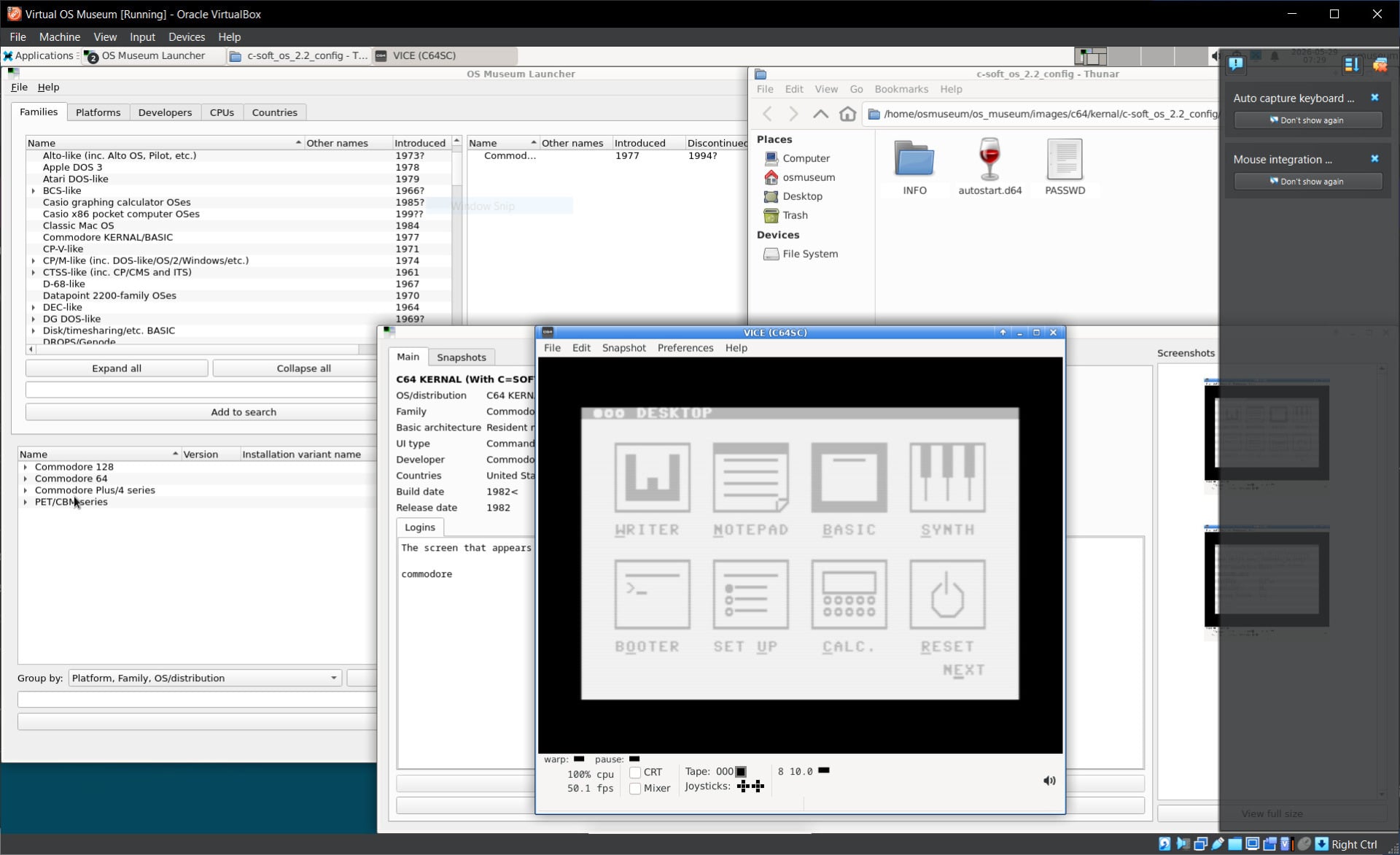
The history of computing is littered with the remains of forgotten operating systems—some rendered obsolete by technological progress, some that never quite captured the public imagination, and some just so aggressively useless that everyone would rather forget they ever existed. But we shouldn’t forget! And happily, there’s a new project devoted to preserving the history of all manner of strange and wonderful OSes: the Virtual OS Museum, a repository of some 1700 operating systems that date back to the dawn of computing as we know it.

This project is all the more remarkable for being the work of one man: Andrew Wartenkin, who has been collecting OS images for over two decades. Of course, Wartenkin didn’t write all the emulation software himself, and he maintains a list of credits to give credit where it’s due. But the work of collecting all the Museum’s material, making sure the various emulations work, and creating a single, fairly seamless point of entry for people interested in exploring them—that’s all Wartenkin.

If you’re interested in having a look yourself, you should know that the Museum isn’t a website where you can just click through to different OS emulations: you need to download and install the project on your computer, and you might need to do a bit of hacking to get it to work.

It’s worth the effort, though, because there’s a ton of fascinating history here to play with. The Museum itself runs in a virtual machine, which seems kinda fitting—it opens in a virtualized Linux installation and presents you with the full list of available operating systems. Did you know someone has written a GUI for the Commodore 64? Neither did I!

There are simulations of ancient mainframes, like the IBM 1130 (yours for the low, low price of $32,280—or $41,230 with a disk drive—back in 1965). And then there are the truly esoteric ones, like the GIER, which, as far as I can tell, was an early transistor-based calculator built in the mid-1960s by Danish company Regnecentralen—most famous for their RC-4000 operating system, which is also included—and sold only in Germany:

Perhaps you’ve always wondered about the IBM 5110, an early attempt at a portable computer? Well, place a stack of cinderblocks on your lap and then boot up the 5110 emulator! which truly stretched the definition of “portable.” Or perhaps you’ve always wondered what it’d be like to play around with the late Terry Davis’s batshit crazy decidedly idiosyncratic TempleOS? Er—well, that one will have to wait, because it doesn’t work at the moment.

Now, as I mentioned, getting started will take a little work. There are two downloads to choose from. As well as the “Full” version, which weighs in at 175 GB when unzipped and contains the entire archive, there’s a “Lite” version, which contains everything you need to get the museum up and running but not the actual OS images themselves—they are downloaded automatically when you choose whichever one you’d like to run. The Lite version is only 21GB unzipped, so unless you’ve got storage space to burn, I’d recommend it over the whole shebang. I’d also recommend using the provided BitTorrent files to download the archive, because they’re a lot faster than the direct download server.

Once you’ve downloaded and extracted the archive, you can move on to getting the Museum up and running. For me, at least, this wasn’t super straightforward, though the issues I encountered are apparently known to Wartenkin and will be fixed in an upcoming version.

For now, the main problem seems to be with VirtualBox’s management of file locations. It needs two large .vdi files to run, and it insists on looking for them in one place only—presumably their original location on Wartenkin’s computer—rather than in the location where you’ve actually extracted them. You can get around this issue by creating a couple of symbolic links to the files. The way to do this will depend on your actual operating system. If you’re on Windows and comfortable with the command prompt, you can use mklink to create links to the files:

mklink "C:\data1\common1\disk_images\os_museum_vm\dist\virtual_os_museum-2026.05.19-lite\VirtualOSMuseum.utm\Data\host_x86.vdi" “[actual path]”

([actual path] is the location of the file on your computer.)

If you’re on macOS or Linux, you can do something similar in the Terminal using the ln command. And if you’re wondering whether you can just create shortcuts to do this: no, you can’t. Well, not on Windows, at least, because I tried it and it doesn’t work.

It’s remarkable that this is all the work of one developer, because it’s often a significant amount of work to get one ancient OS working under emulation, let alone hundreds of them. With that said, I do hope that the project arrives at a place where it’s a little more user-friendly, because it’s a hugely valuable endeavor, and it’d be great if it were easy for casual users to explore with a minimum of friction. We look forward to future updates!